Machine Learning Overview

Applied Machine Learning

Jameson > Hendrik > Calvin

Agenda

  1. Course Overview
  2. Review of Regression
  3. Dinner Break
  4. Classification and Ethics
  5. Basic Feature Engineering
  6. Vocabulary

Course Overview

Expectations and assignments

  1. Homework assignments
  2. Exam
  3. Modeling Project
  4. Course Policies
  5. My expectations for you

Homeworks

  • Create a .rmd or ideally .qmd file.
  • Render it to .html.
  • Publish both files on GitHub Pages.
  • Send me a link from your @willamette.edu address.
  • Consider sharing on e.g. your LinkedIn, or not.
  • You may use R or Python
    • We introduce Python in a special King Day video lecture.

Midterm Exam

  • I need to measure if I’m teaching well.
  • Low stress for you.

Modeling Project

  • Three part group project.
  • We’ll get there.

Course Policies

  • Don’t do anything you wouldn’t do in 501/502/504
  • LLMs are approved for use in this course.

My Expectations

  • Professional carriage and mutual respect are paramount.
  • Technical skills are secondary to interpersonal.
  • Technical skills support interpersonal by facilitating insight.

About me

  • BA Mathematics, BS Computer Science (UChicago)
  • MS, PhD Computer Science (UNC Chapel Hill)
  • Data mining, formal analysis, complex models
  • Joined Willamette 2021

About you?

  • Background
  • Goals for this program and/or course

Basic concepts in Machine Learning

  • What is a data scientist?
  • What is machine learning?
  • What is the role of judgment in machine learning?
  • What are the differences between machine learning, statistics and econometrics?
  • When is “mere” correlation enough? When is it not?

Packages

  • Today I use the following libraries:
local({r <- getOption("repos")
       r["CRAN"] <- "https://cran.r-project.org" 
       options(repos=r)
})
# New?
install.packages("tidyverse")
package 'tidyverse' successfully unpacked and MD5 sums checked

The downloaded binary packages are in
    C:\Users\cd-desk\AppData\Local\Temp\Rtmpa25X7Y\downloaded_packages
install.packages("moderndive")
package 'moderndive' successfully unpacked and MD5 sums checked

The downloaded binary packages are in
    C:\Users\cd-desk\AppData\Local\Temp\Rtmpa25X7Y\downloaded_packages
install.packages("caret")
package 'caret' successfully unpacked and MD5 sums checked

The downloaded binary packages are in
    C:\Users\cd-desk\AppData\Local\Temp\Rtmpa25X7Y\downloaded_packages
install.packages("dslabs")
package 'dslabs' successfully unpacked and MD5 sums checked

The downloaded binary packages are in
    C:\Users\cd-desk\AppData\Local\Temp\Rtmpa25X7Y\downloaded_packages
# Just for the slides
install.packages("thematic")
package 'thematic' successfully unpacked and MD5 sums checked

The downloaded binary packages are in
    C:\Users\cd-desk\AppData\Local\Temp\Rtmpa25X7Y\downloaded_packages
  • You will have some but perhaps not others.

Libraries

  • I’ll just include them upfront.
library(tidyverse)
library(moderndive)
library(caret)
library(dslabs)
# Just for the slides
library(thematic)
theme_set(theme_dark())
thematic_rmd(bg = "#111", fg = "#eee", accent = "#eee")

Setup

  • We will work with a wine dataset that is enormous.
    • Just to render a bit quickly, take a sample.
    • You are welcome to work with the full dataset!
wine <- readRDS(gzcon(url("https://cd-public.github.io/D505/dat/wine.rds")))
wine <- wine %>% drop_na(points, price)
summary(wine)
       id           country          description        designation       
 Min.   :     1   Length:89556       Length:89556       Length:89556      
 1st Qu.: 32742   Class :character   Class :character   Class :character  
 Median : 65613   Mode  :character   Mode  :character   Mode  :character  
 Mean   : 65192                                                           
 3rd Qu.: 97738                                                           
 Max.   :129970                                                           
     points           price           province           region_1        
 Min.   : 80.00   Min.   :   4.00   Length:89556       Length:89556      
 1st Qu.: 87.00   1st Qu.:  17.00   Class :character   Class :character  
 Median : 89.00   Median :  25.00   Mode  :character   Mode  :character  
 Mean   : 88.65   Mean   :  35.56                                        
 3rd Qu.: 91.00   3rd Qu.:  42.00                                        
 Max.   :100.00   Max.   :3300.00                                        
   region_2         taster_name        taster_twitter_handle    title          
 Length:89556       Length:89556       Length:89556          Length:89556      
 Class :character   Class :character   Class :character      Class :character  
 Mode  :character   Mode  :character   Mode  :character      Mode  :character  


   variety             winery               year     
 Length:89556       Length:89556       Min.   :1995  
 Class :character   Class :character   1st Qu.:2010  
 Mode  :character   Mode  :character   Median :2012  
                                       Mean   :2011  
                                       3rd Qu.:2014  
                                       Max.   :2015  

Review of Regression

Single Variable

  • Pick the poshest province.
wine <- wine %>%
  mutate(bordeaux = (province == "Bordeaux"))
wine <- wine %>% drop_na(bordeaux)
top_n(wine, 10, bordeaux)
# A tibble: 3,774 × 16
      id country description designation points price province region_1 region_2
   <dbl> <chr>   <chr>       <chr>        <dbl> <dbl> <chr>    <chr>    <chr>   
 1    53 France  Fruity and… La Fleur d…     85    15 Bordeaux Bordeau… <NA>    
 2   136 France  This wine'… <NA>            91    50 Bordeaux Saint-É… <NA>    
 3   419 France  A smooth, … <NA>            89    20 Bordeaux Graves   <NA>    
 4   477 France  An interes… <NA>            92    65 Bordeaux Pomerol  <NA>    
 5   573 France  Fruity and… <NA>            89    14 Bordeaux Bordeau… <NA>    
 6   575 France  This is a … <NA>            89    14 Bordeaux Bordeau… <NA>    
 7   576 France  From a Gra… Les Terras…     89    37 Bordeaux Saint-É… <NA>    
 8   578 France  A ripe per… Château Je…     89    15 Bordeaux Bordeaux <NA>    
 9   792 France  The 45% Ca… La Sérénit…     90    30 Bordeaux Médoc    <NA>    
10   795 France  This is th… Divin de C…     90    35 Bordeaux Saint-É… <NA>    
# ℹ 3,764 more rows
# ℹ 7 more variables: taster_name <chr>, taster_twitter_handle <chr>,
#   title <chr>, variety <chr>, winery <chr>, year <dbl>, bordeaux <lgl>

Regress

  • Take a quick regression model over the wine.
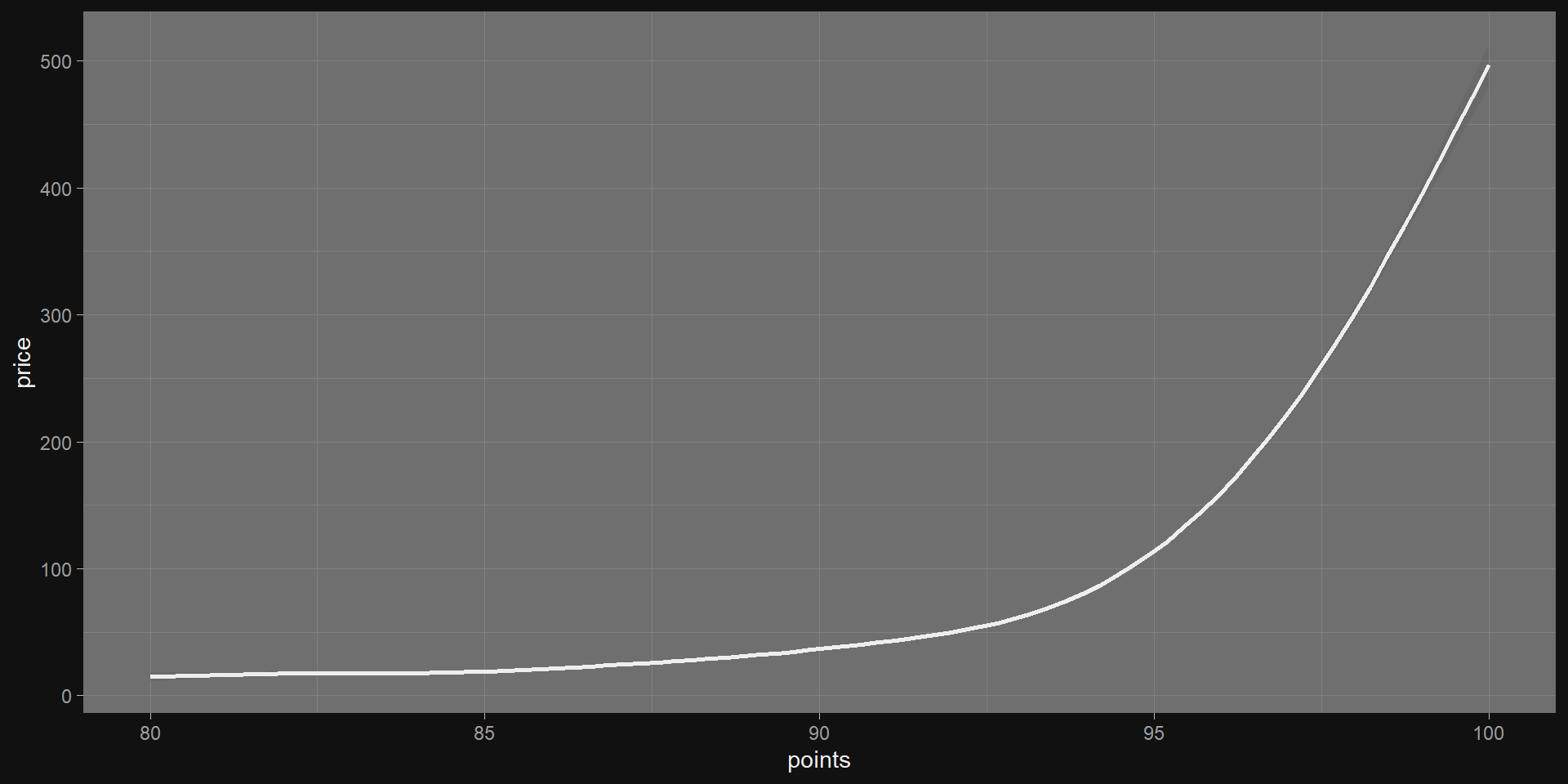
m1 <- lm(price ~ points, data = wine)
get_regression_table(m1)
# A tibble: 2 × 7
  term      estimate std_error statistic p_value lower_ci upper_ci
  <chr>        <dbl>     <dbl>     <dbl>   <dbl>    <dbl>    <dbl>
1 intercept  -489.       3.97      -123.       0  -497.    -482.  
2 points        5.92     0.045      132.       0     5.83     6.01

Let’s draw it

Multiple regression

m2 <- lm(price ~ points + bordeaux, data = wine)
get_regression_table(m2)
# A tibble: 3 × 7
  term         estimate std_error statistic p_value lower_ci upper_ci
  <chr>           <dbl>     <dbl>     <dbl>   <dbl>    <dbl>    <dbl>
1 intercept     -492.       3.97     -124.        0  -500.    -484.  
2 points           5.95     0.045     133.        0     5.86     6.03
3 bordeauxTRUE     8.70     0.661      13.2       0     7.41    10.0 

Let’s draw it

How about with an interaction?

m3 <- lm(price ~ points * bordeaux, data = wine)
get_regression_table(m3)
# A tibble: 4 × 7
  term                estimate std_error statistic p_value lower_ci upper_ci
  <chr>                  <dbl>     <dbl>     <dbl>   <dbl>    <dbl>    <dbl>
1 intercept            -461.       4.04     -114.        0  -469.    -453.  
2 points                  5.60     0.045     123.        0     5.51     5.69
3 bordeauxTRUE         -666.      18.8       -35.5       0  -703.    -629.  
4 points:bordeauxTRUE     7.66     0.213      36.0       0     7.24     8.07

Let’s draw it

Model diagnostics

get_regression_summaries(m1)
# A tibble: 1 × 9
  r_squared adj_r_squared   mse  rmse sigma statistic p_value    df  nobs
      <dbl>         <dbl> <dbl> <dbl> <dbl>     <dbl>   <dbl> <dbl> <dbl>
1     0.164         0.164 1579.  39.7  39.7    17497.       0     1 89503
get_regression_summaries(m2)
# A tibble: 1 × 9
  r_squared adj_r_squared   mse  rmse sigma statistic p_value    df  nobs
      <dbl>         <dbl> <dbl> <dbl> <dbl>     <dbl>   <dbl> <dbl> <dbl>
1     0.165         0.165 1576.  39.7  39.7     8852.       0     2 89503
get_regression_summaries(m3)
# A tibble: 1 × 9
  r_squared adj_r_squared   mse  rmse sigma statistic p_value    df  nobs
      <dbl>         <dbl> <dbl> <dbl> <dbl>     <dbl>   <dbl> <dbl> <dbl>
1     0.177         0.177 1553.  39.4  39.4     6418.       0     3 89503

Moving to an ML framework

Split sample using Caret

set.seed(505)
train_index <- createDataPartition(wine$price, times = 1, p = 0.8, list = FALSE)
train <- wine[train_index, ]
test <- wine[-train_index, ]
head(test)
# A tibble: 6 × 16
     id country description  designation points price province region_1 region_2
  <dbl> <chr>   <chr>        <chr>        <dbl> <dbl> <chr>    <chr>    <chr>   
1     8 Germany Savory drie… Shine           87    12 Rheinhe… <NA>     <NA>    
2    19 US      Red fruit a… <NA>            87    32 Virginia Virginia <NA>    
3    20 US      Ripe aromas… Vin de Mai…     87    23 Virginia Virginia <NA>    
4    28 Italy   Aromas sugg… Mascaria B…     87    17 Sicily … Cerasuo… <NA>    
5    59 US      Aromas of c… <NA>            86    55 Washing… Columbi… Columbi…
6    61 Italy   This densel… Prugneto        86    17 Central… Romagna  <NA>    
# ℹ 7 more variables: taster_name <chr>, taster_twitter_handle <chr>,
#   title <chr>, variety <chr>, winery <chr>, year <dbl>, bordeaux <lgl>

Compare RMSE across models

  • Retrain on models on the training set
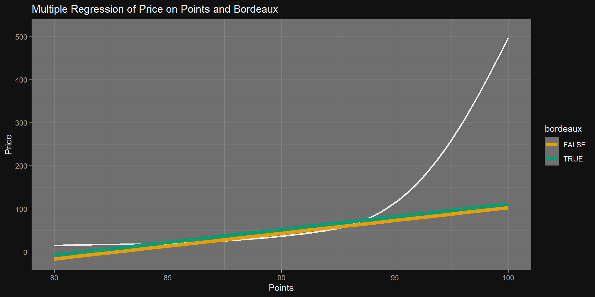
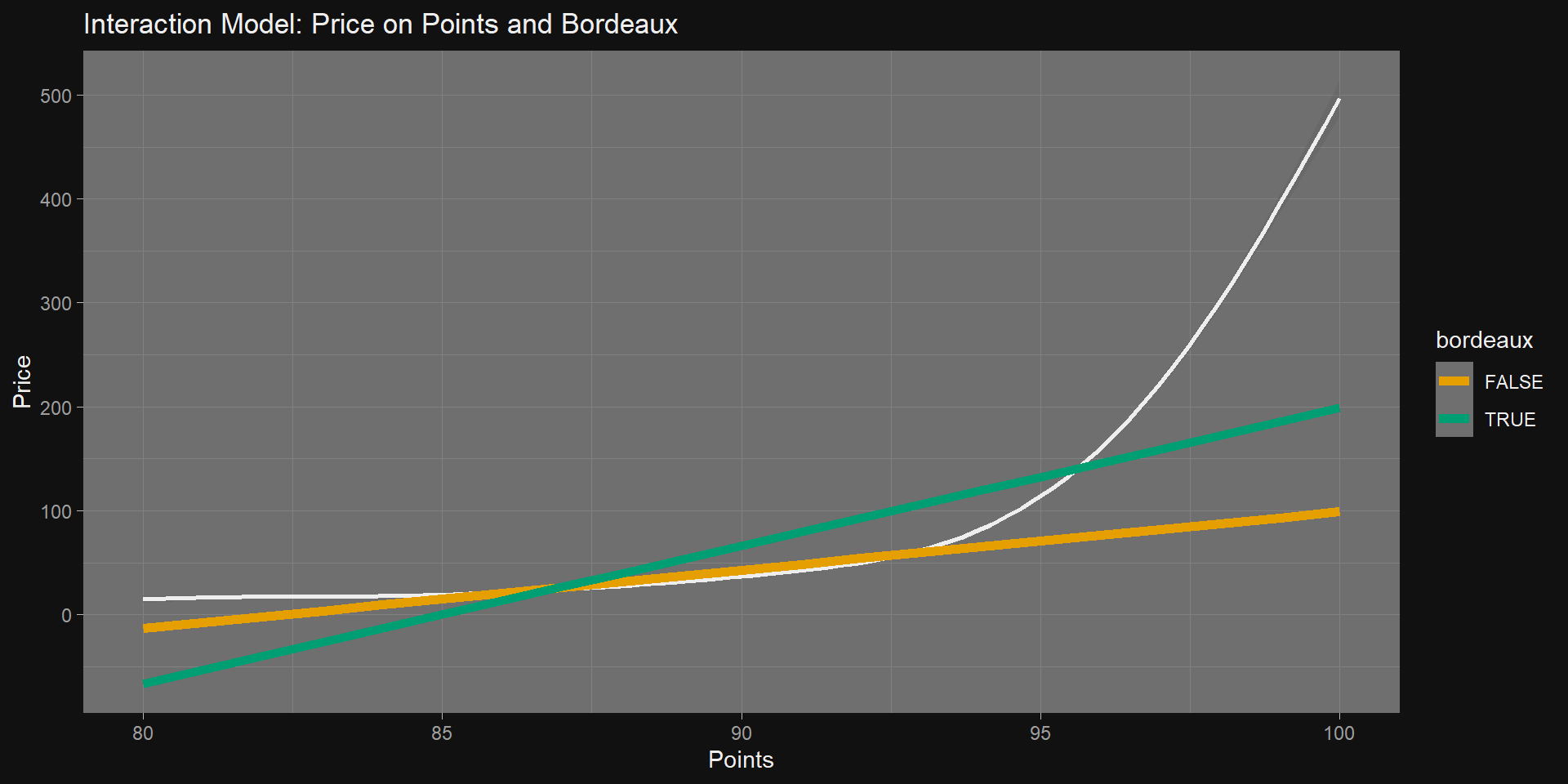
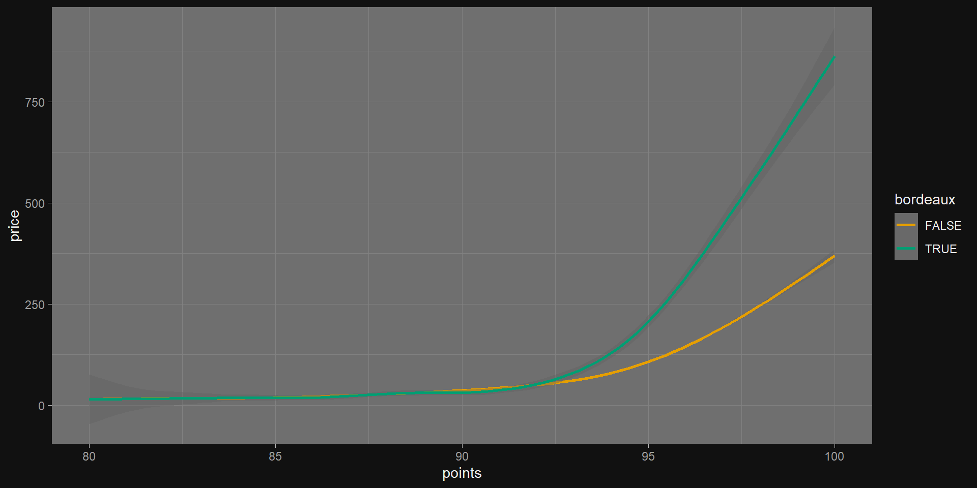
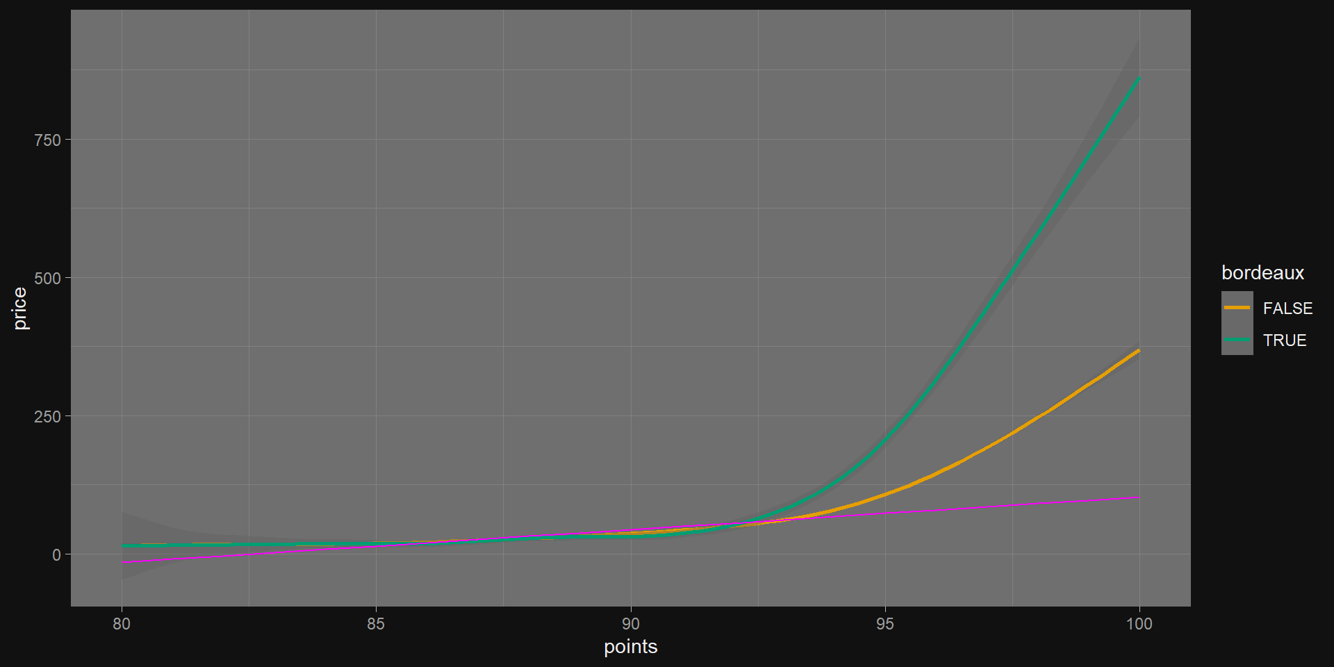
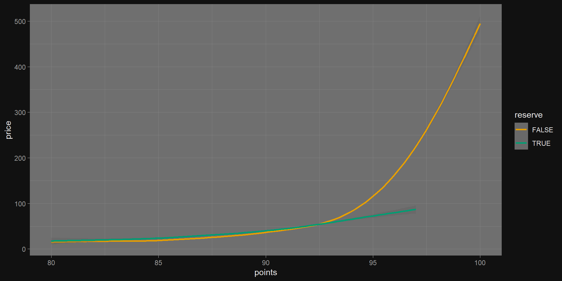
ms <- list(
  lm(price ~ points, data = train),
  lm(price ~ points + bordeaux, data = train),
  lm(price ~ points * bordeaux, data = train)
)
  • Test them all under the same conditions.
map(ms, function(m) {
  get_regression_points(m, newdata = test) %>%
    drop_na(residual) %>%
    mutate(sq_residuals = residual^2) %>%
    summarize(rmse = sqrt(mean(sq_residuals))) %>%
    pluck("rmse")
}) %>% unlist()
[1] 36.00999 36.00970 35.85276

Group Exercise (30m)

  1. Load the wine data set
  2. Visualize the relationship of points and price
  3. Bonus: Color the observations based on whether the wine is from Bordeaux
  4. Bonus+: Include regression lines
  5. Bonus++: Pick a non-Bordeaux category.

Plot

  • Points vs. price.
wine %>%
  ggplot(aes(x = points, y = price)) +
  geom_smooth()

Bonus

  • Color the Bordeaux region.
wine %>%
  ggplot(aes(x = points, y = price, color = bordeaux)) +
  geom_smooth()

Bonus+

  • Include regression lines
wine %>%
  mutate(m = predict(lm(price ~ points, data = wine))) %>%
  ggplot() +
  geom_smooth(aes(x = points, y = price, color = bordeaux)) +
  geom_line(aes(x = points, y = m), colour = "magenta")

Bonus++

  • Let’s look at “reserve”.
wine %>%
  mutate(reserve = grepl("Reserve", designation)) %>%
  ggplot(aes(x = points, y = price, color = reserve)) +
  geom_smooth()

Bonus

  • Anglophones to Francophiles.
wine %>%
  mutate(reservæ = grepl("Reserve", designation, ignore.case = TRUE) |
    grepl("Reserva", designation, ignore.case = TRUE)) %>%
  ggplot(aes(x = points, y = price, color = reservæ)) +
  geom_smooth()

RჂservæ

  • Cross the Alps.
wine %>%
  mutate(rჂservæ = grepl("Reserve|Reserva|Riserva", designation, ignore.case = TRUE)) %>%
  ggplot(aes(x = points, y = price, color = rჂservæ)) +
  geom_smooth()

Dinner break

  • On “rჂservæ”
    • Ie or Iota (asomtavruli Ⴢ, nuskhuri ⴢ, mkhedruli ჲ, mtavruli Ჲ) is the 15th letter of the three Georgian scripts

Classification and Ethics

The math of it…

  • Suppose I’m trying to predict sex based on height.
    • Don’t do this in real life (obviously).
  • We start by
    • defining the outcome and predictors, and…
    • creating training and test data.

Partition our Data

data(heights) # from library(dslabs)
y <- heights$sex
x <- heights$height
set.seed(505)
test_index <- createDataPartition(y, list = FALSE)
test_set <- heights[test_index, ]
train_set <- heights[-test_index, ]
summary(heights)
     sex          height     
 Female:238   Min.   :50.00  
 Male  :812   1st Qu.:66.00  
              Median :68.50  
              Mean   :68.32  
              3rd Qu.:71.00  
              Max.   :82.68  

Note: this vignette is adapted from this book

Guessing

  • Let’s start by developing the simplest possible machine algorithm: guessing the outcome.
y_hat <- sample(c("Male", "Female"), length(test_index), replace = TRUE)

Recall:

Y hat (written ŷ ) is the predicted value of y (the dependent variable) in a regression equation. It can also be considered to be the average value of the response variable.

Accuracy

  • The overall accuracy is simply defined as the overall proportion that is predicted correctly:
mean(y_hat == test_set$sex)
[1] 0.5180952
  • What would we have expected the accuracy to be?
    • What much would we have expected accuracy to deviate from that expectionation?

Let’s do better…

summary <- heights %>%
  group_by(sex) %>%
  summarize(mean(height), sd(height))
summary
# A tibble: 2 × 3
  sex    `mean(height)` `sd(height)`
  <fct>           <dbl>        <dbl>
1 Female           64.9         3.76
2 Male             69.3         3.61

A simple predictive model

  • Idea: Predict "Male" if observation is within 2 standard deviations
male_mean_less_2sd <- summary[2, ]["mean(height)"] - 2 * summary[2, ]["sd(height)"]

y_hat <- ifelse(x > male_mean_less_2sd, "Male", "Female") %>%
  factor(levels = levels(test_set$sex))

c(male_mean_less_2sd, mean(y == y_hat))
$`mean(height)`
[1] 62.09271

[[2]]
[1] 0.7733333
  • The accuracy goes up from ~0.50 to about ~0.80!!

Let’s optimize

cutoff <- seq(61, 70)
get_accuracy <- function(x) {
  y_hat <- ifelse(train_set$height > x, "Male", "Female")
  mean(y_hat == train_set$sex)
}
accuracy <- map(cutoff, get_accuracy)

unlist(accuracy)
 [1] 0.7752381 0.7866667 0.8152381 0.8342857 0.8209524 0.7904762 0.7314286
 [8] 0.6819048 0.5961905 0.5104762
  • Most are much higher than 0.5!!

Let’s take a gander

  • Easier for me to see it.
plot(cutoff, accuracy)

Optimal Cutoff

best_cutoff <- cutoff[which.max(accuracy)]
best_cutoff
[1] 64
  • Should we be cutting at an integer?

Apply & Evaluate

y_hat <- ifelse(test_set$height > best_cutoff, "Male", "Female")
mean(y_hat == test_set$sex)
[1] 0.8190476

Confusion matrix

table(predicted = y_hat, actual = test_set$sex) %>%
  as.data.frame() %>%
  ggplot(aes(x = predicted, y = actual)) +
  geom_tile(aes(fill = Freq), color = "white") +
  scale_fill_gradient(low = "white", high = "blue") +
  geom_text(aes(label = Freq), vjust = "center", color = "black", size = 24) +
  labs(title = "Confusion Matrix", x = "Predicted", y = "Actual")

Accuracy by sex

test_set %>%
  mutate(y_hat = y_hat) %>%
  group_by(sex) %>%
  summarize(accuracy = mean(y_hat == sex))
# A tibble: 2 × 2
  sex    accuracy
  <fct>     <dbl>
1 Female    0.445
2 Male      0.929


It’s raining men.

Debrief

heights %>%
  ggplot() +
  geom_boxplot(aes(height, sex))

slices <- heights %>%
  group_by(sex) %>%
  tally()
pie(slices$n, labels = slices$sex)

Moral of the story

Other ethical issues

  • Demographic data
  • Profit optimizing
  • Autonomous cars
  • Recommendation engines
  • Fair housing
  • Criminal sentencing
  • Choice of classification model
  • Drone warfare

Jameson on Ethics

Reasonable people will disagree over subtle matters of right and wrong… thus, the important part of data ethics is committing to consider the ethical consequences of your choices.

The difference between “regular” ethics and data ethics is that algorithms scale really easily. Thus, seemingly small decisions can have wide-ranging impact.

Calvin on Ethics

No ethical [computation] under capitalism

  • Usage of data | computing is ethicial iff it challenges rather than strengthens existing power relations.

Vocabulary

ML Terms

Definition of ML: using data to find a function that minimizes prediction error.

  • Features
  • Variables
  • Outcome variable
  • Regression
  • RMSE
  • Classification
  • Confusion matrix
  • Split Samples

Features

  • Definition: Individual measurable properties or attributes of data.
  • Example: Age, income, and education level in a dataset predicting loan approval.

Variables

  • Definition: Data points that can change and impact predictions.
  • Example: Independent variables like weather, and dependent variables like crop yield.

Outcome Variable

  • Definition: The target or dependent variable the model predicts.
  • Example: Predicting “passed” or “failed” for a student’s exam result.

Features vs. Variables

  • Features: Inputs to the model, often selected or engineered from raw data.
    • Example: “Average monthly income” derived from raw transaction data.
  • Variables: Broader term encompassing both inputs (independent) and outputs (dependent).
    • Example: “House price” (dependent variable) depends on features like size and location.

Regression

  • Definition: Statistical method to model the relationship between variables.
  • Example: Linear regression predicts house prices based on size and location.

RMSE (Root Mean Square Error)

  • Definition: A metric to measure prediction accuracy by averaging squared errors.
  • Example: Lower RMSE in predicting drug response indicates a better model fit.

Classification

  • Definition: Task of predicting discrete categories or labels.
  • Example: Classifying emails as “spam” or “not spam.”
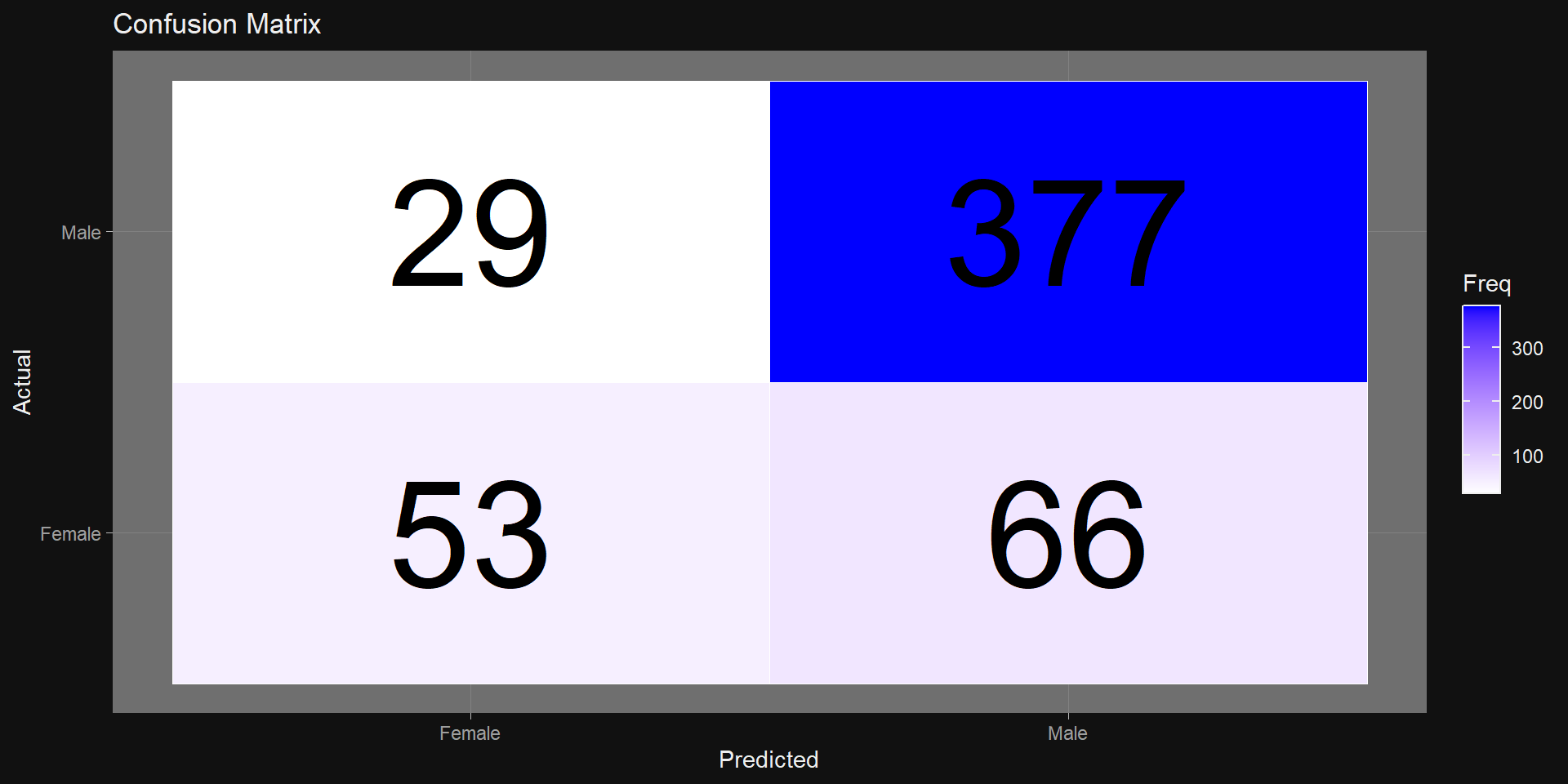
Confusion Matrix

  • Definition: A table showing model performance in classification tasks.
  • Example: Matrix rows show true values; columns show predicted outcomes.

Split Samples

  • Definition: Dividing data into training and testing subsets for validation.
  • Example: 80% training, 20% testing ensures unbiased model evaluation.
test_set <- heights[test_index, ]
train_set <- heights[-test_index, ]

Bonus Slides:
Precision-recall

Precision-recall tradeoff

  • Precision: TP / (TP + FP)
  • Recall: TP / (TP + FN)
  • Imagine I have a fraud-detection model that gives 1,000 credit card transactions each a risk score.

Precision-recall tradeoff

  • Imagine I have a fraud-detection model that gives 1,000 credit card transactions each a risk score.
  • The company chooses a risk score cutoff of 77 (for some reason).
  • There are 18 transactions with risk above 77. 12 are actually fraud. 20 fraudulent transactions have risk below 77.
  • What are precision, recall, and accuracy?

Precision-recall Exercise

  • Precision: TP / (TP + FP)
  • Recall: TP / (TP + FN)
  • 1,000 credit card transactions
  • The company chooses a risk score cutoff of 77
  • There are 18 transactions with risk above 77.
    • 12 are actually fraud.
    • 20 fraudulent transactions have risk below 77.
  • TODO Calculate precision, recall, and accuracy.

Solutions

- Definitions
  - Precision: TP / (TP + FP)
  - Recall:    TP / (TP + FN)
- Computation
  - Precision: 12 / (12 + 06)  ~= 67%
  - Recall:    12 / (12 + 20)  ~= 38%
  - Accuracy: (12 + 962)/1000  ~= 97%

Precision-recall tradeoff

  • Precision: TP / (TP + FP)
  • Recall: TP / (TP + FN)
  • Image: Hands-on machine learning, A. Geron