Feature Engineering & Variable Selection

Applied Machine Learning

Jameson > Hendrik > Calvin

Agenda

1. Review of Homework 1
2. Feature Engineering I
3. Dinner Break
4. The Caret framework
5. Vocabulary

Packages

• Today I use the following libraries:

local({r <- getOption("repos")
       r["CRAN"] <- "https://cran.r-project.org" 
       options(repos=r)
})
# Old
# install.packages("tidyverse")
# install.packages("caret")
# New?
install.packages("fastDummies")
# Just for the slides
# install.packages("thematic")

• You will have some but perhaps not others.

Libraries

• I’ll just include them upfront.

library(tidyverse)
library(caret)
library(fastDummies)
# Just for the slides
library(thematic)
theme_set(theme_dark())
thematic_rmd(bg = "#111", fg = "#eee", accent = "#eee")

Setup

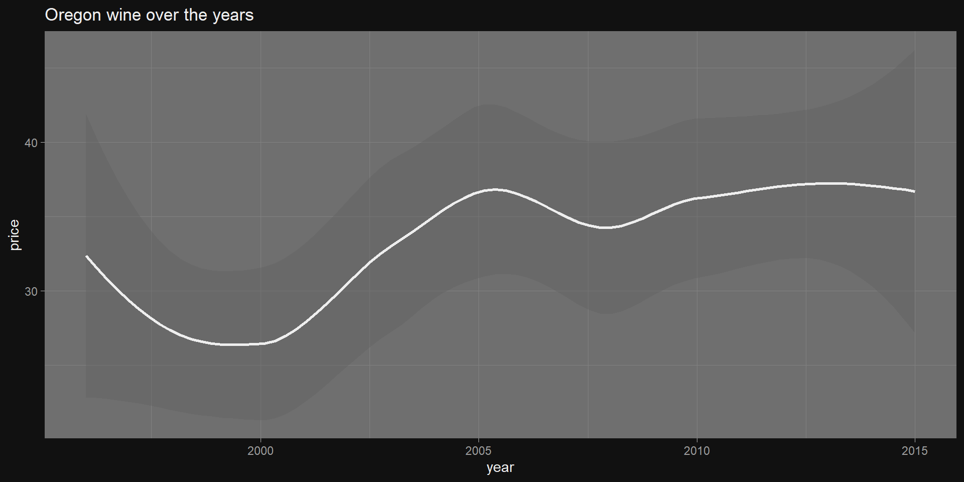
• We will work with a wine dataset that is enormous.
  • Just to render a bit quickly, take a sample.
  • You are welcome to work with the full dataset!

wine <- readRDS(gzcon(url("https://cd-public.github.io/D505/dat/wine.rds")))
# performance concession
# wall <- wine
# wine = wall[sample(nrow(wall), 100), ]
summary(wine)

       id           country          description        designation       
 Min.   :     1   Length:89556       Length:89556       Length:89556      
 1st Qu.: 32742   Class :character   Class :character   Class :character  
 Median : 65613   Mode  :character   Mode  :character   Mode  :character  
 Mean   : 65192                                                           
 3rd Qu.: 97738                                                           
 Max.   :129970                                                           
     points           price           province           region_1        
 Min.   : 80.00   Min.   :   4.00   Length:89556       Length:89556      
 1st Qu.: 87.00   1st Qu.:  17.00   Class :character   Class :character  
 Median : 89.00   Median :  25.00   Mode  :character   Mode  :character  
 Mean   : 88.65   Mean   :  35.56                                        
 3rd Qu.: 91.00   3rd Qu.:  42.00                                        
 Max.   :100.00   Max.   :3300.00                                        
   region_2         taster_name        taster_twitter_handle    title          
 Length:89556       Length:89556       Length:89556          Length:89556      
 Class :character   Class :character   Class :character      Class :character  
 Mode  :character   Mode  :character   Mode  :character      Mode  :character  
                                                                               
                                                                               
                                                                               
   variety             winery               year     
 Length:89556       Length:89556       Min.   :1995  
 Class :character   Class :character   1st Qu.:2010  
 Mode  :character   Mode  :character   Median :2012  
                                       Mean   :2011  
                                       3rd Qu.:2014  
                                       Max.   :2015  

Feature Engineering

Group Exercise (30m)

1. Identify 3 “interesting” features of the wine dataset
2. Bonus
   • ∃ Critic “Roger Voss”
   • ∃ a wine varietal(s) “Voss” seems to dislike
   • Find said varietal.

Categorical vs. Continuous

• What is a categorical variable?
• What is a continuous variable?
• Why visualize at the data before modeling it?

Categorical Example 1

wine %>%
  mutate(roger = taster_name == "Roger Voss") %>%
  mutate(pinot_gris = variety == "Pinot Gris") %>%
  drop_na(roger) %>%
  group_by(roger, pinot_gris) %>%
  summarize(points = mean(points)) %>%
  ggplot() +
  aes(pinot_gris, points, color = roger) +
  geom_line(aes(group = roger), size = 2)

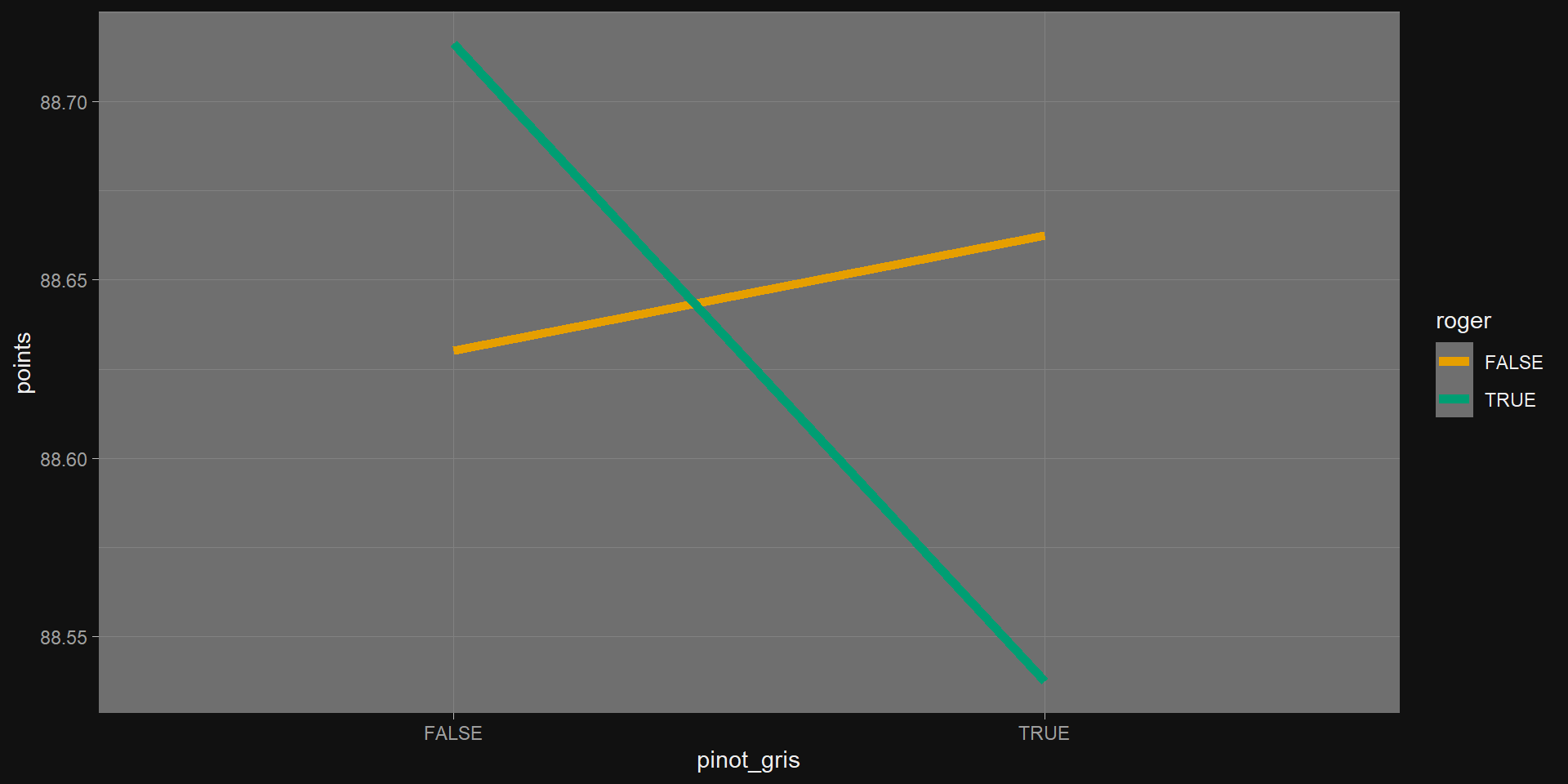
Categorical Example 2

wine %>%
  filter(province == "Oregon") %>%
  group_by(year) %>%
  summarize(price = mean(price)) %>%
  ggplot(aes(year, price)) +
  geom_smooth() +
  labs(title = "Oregon wine over the years")

Exercise (15 min)

1. Group by winery and year, Find:
   • The average score, and
   • Number of reviews.
2. Find year-on-year change in score by winery.
3. How might you use this in prediction?
   • What kind of problem might it help with?

Year-on-Year Change Example

wine %>%
  group_by(winery, year) %>%
  summarize(avg_score = mean(points), num_reviews = n_distinct(id)) %>%
  select(year, winery, num_reviews, avg_score) %>%
  arrange(winery, year) %>%
  mutate(score_change = avg_score - lag(avg_score)) %>%
  drop_na(score_change) %>%
  summarize(mean(score_change))

# A tibble: 8,409 × 2
   winery           `mean(score_change)`
   <chr>                           <dbl>
 1 100 Percent Wine               -1.5  
 2 12 Linajes                     -0.333
 3 12C Wines                       1.25 
 4 14 Hands                       -0.111
 5 2 Lads                         -2.25 
 6 2 Up                            0    
 7 21 Grams                        1    
 8 29 & Oak Wines                 -2    
 9 2Hawk                           0.75 
10 2Plank                         -1.25 
# ℹ 8,399 more rows

Dummy Variables

• What are Dummy Variables?:
  • Represent categories as 0s and 1s for models.
    
• Why Use Dummy Variables?:
  • Handle categorical data in numerical algorithms.
    
• Avoid Dummy Trap:
  • Drop one column to prevent multicollinearity.

Many vs Few Dummies

• Few Dummies:
  • Simplifies models, risks losing fine-grained patterns.
• Many Dummies:
  • Captures detailed trends, increases model complexity.
• Key Decision:
  • Balance interpretability and predictive power.

“fastDummies” Package

• Purpose:
  • Quickly create dummy variables in R datasets.
• Key Functions:
  • dummy_cols() adds dummy columns efficiently.
• Features:
  • Handles multiple columns and missing data flexibly.

Few Dummies

wine %>%
  select(taster_name) %>%
  dummy_cols() %>% # library(fastDummies)
  select(1:4) %>%
  head()

# A tibble: 6 × 4
  taster_name        `taster_name_Alexander Peartree` taster_name_Anna Lee C. …¹
  <chr>                                         <int>                      <int>
1 Roger Voss                                        0                          0
2 Paul Gregutt                                      0                          0
3 Alexander Peartree                                1                          0
4 Paul Gregutt                                      0                          0
5 Michael Schachner                                 0                          0
6 Kerin O’Keefe                                     0                          0
# ℹ abbreviated name: ¹​`taster_name_Anna Lee C. Iijima`
# ℹ 1 more variable: `taster_name_Anne Krebiehl MW` <int>

Many Dummies

wine %>%
  select(variety) %>%
  mutate(variety = fct_lump(variety, 4)) %>%
  dummy_cols() %>%
  head()

# A tibble: 6 × 6
  variety    variety_Cabernet Sauvigno…¹ variety_Chardonnay `variety_Pinot Noir`
  <fct>                            <int>              <int>                <int>
1 Other                                0                  0                    0
2 Other                                0                  0                    0
3 Other                                0                  0                    0
4 Pinot Noir                           0                  0                    1
5 Other                                0                  0                    0
6 Other                                0                  0                    0
# ℹ abbreviated name: ¹​`variety_Cabernet Sauvignon`
# ℹ 2 more variables: `variety_Red Blend` <int>, variety_Other <int>

Other types of engineered categorical features…

• Words or phrases in text
• A given time period
• An arbitrary numerical cut-off
• Demographic variables

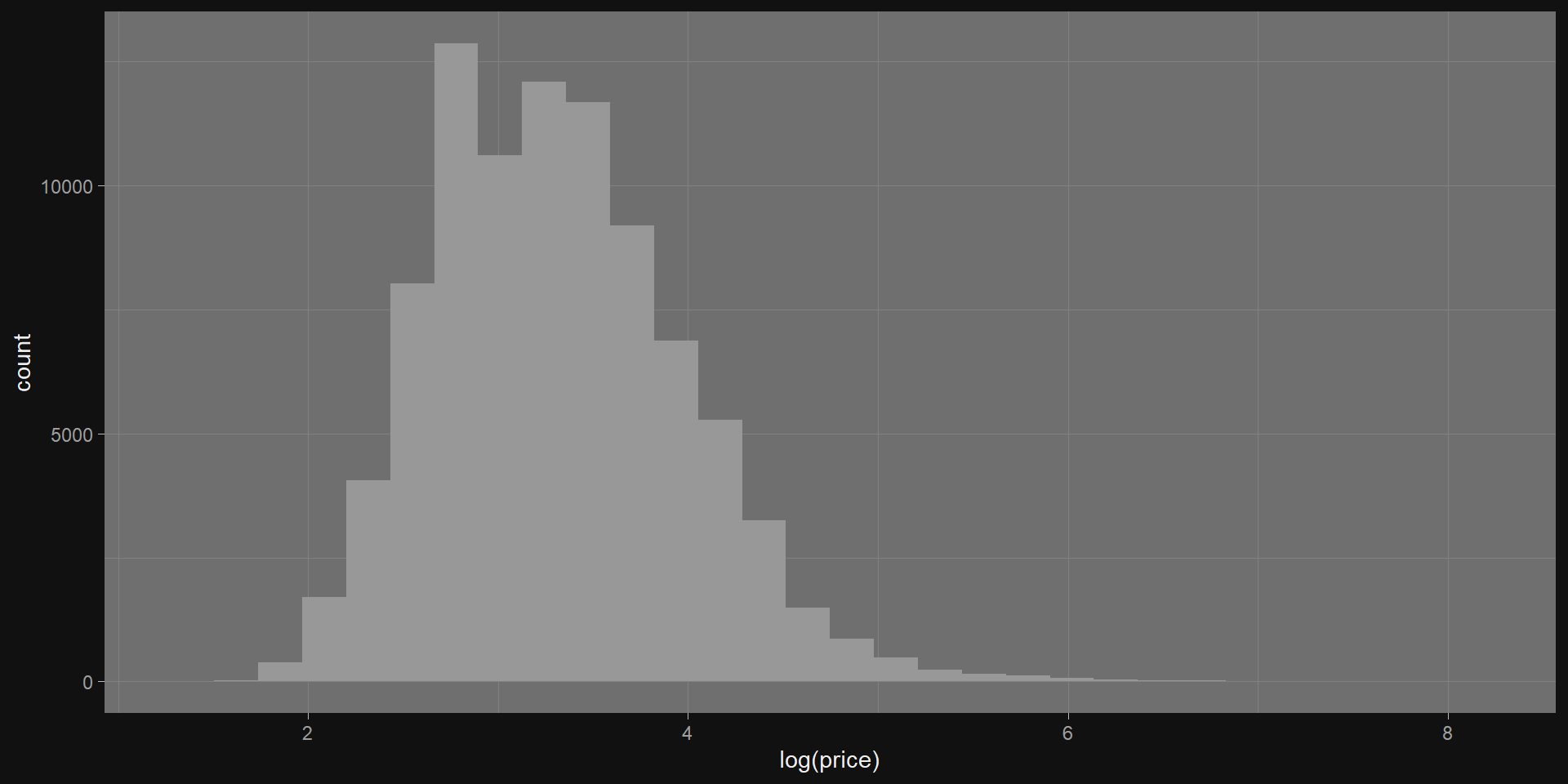
What about numerical features?

wine %>%
  ggplot(aes(price)) +
  geom_histogram()

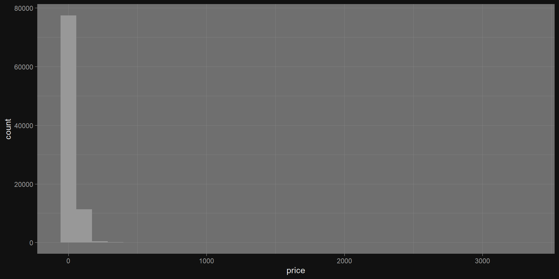
Take the natural log

wine %>%
  ggplot(aes(log(price))) +
  geom_histogram()

Standardizing

• Create a common scale across variables.
  • Mean-centering \(x-\bar{x}\)
  • Scaling: \(x/std(x)\)
• Helps reduce bias when interactions are included.
  • (i.e. eliminates variance inflation).

Other transformations.

• I use logs > 95% of the time, standarizing ~40%.
• There are many other transformations:
  • YoY, QoQ, etc. (absolute and percent)
  • log
  • polynomial transforms
  • lags!

Standardize

• list(normalized = ~(scale(.) %>% as.vector)): :
  • scale(.): Standardizes the “points” column.
  • %>% as.vector: Converts back to a vector.

wine %>% mutate_at("points", list(standardized = ~ (scale(.) %>% as.vector())))

# A tibble: 89,556 × 16
      id country description designation points price province region_1 region_2
   <dbl> <chr>   <chr>       <chr>        <dbl> <dbl> <chr>    <chr>    <chr>   
 1     1 Portug… This is ri… Avidagos        87    15 Douro    <NA>     <NA>    
 2     2 US      Tart and s… <NA>            87    14 Oregon   Willame… Willame…
 3     3 US      Pineapple … Reserve La…     87    13 Michigan Lake Mi… <NA>    
 4     4 US      Much like … Vintner's …     87    65 Oregon   Willame… Willame…
 5     5 Spain   Blackberry… Ars In Vit…     87    15 Norther… Navarra  <NA>    
 6     6 Italy   Here's a b… Belsito         87    16 Sicily … Vittoria <NA>    
 7     7 France  This dry a… <NA>            87    24 Alsace   Alsace   <NA>    
 8     8 Germany Savory dri… Shine           87    12 Rheinhe… <NA>     <NA>    
 9     9 France  This has g… Les Natures     87    27 Alsace   Alsace   <NA>    
10    10 US      Soft, supp… Mountain C…     87    19 Califor… Napa Va… Napa    
# ℹ 89,546 more rows
# ℹ 7 more variables: taster_name <chr>, taster_twitter_handle <chr>,
#   title <chr>, variety <chr>, winery <chr>, year <dbl>, standardized <dbl>

Interaction effects

This chapter has a good overview of interactions.

• Start with domain knowledge.
• Use visualizations.
• 3-way interactions exist, but are rare.
  • If you suspect a 3-way, also suspect your suspicions.
  • Complexity increases exponentially in “ways”.
  • These are notoriously hard to explain.

Dinner (and virtual high fives)

Le Bibliothèques caret

Philosophy

Types of resampling

• V-fold Cross-Validation
  • Divides data into \(k\) folds, trains on \(k−1\) folds, validates on the remaining fold, for all folds.
• Monte Carlo Cross-Validation
  • Randomly splits data into training and validation sets multiple times, averaging results for evaluation.
• The Bootstrap
  • Uses resampling with replacement to estimate model accuracy and variability.

Setup the Dataframe

• Follow this link for the full documentation on caret.

wino <- wine %>% # 3 engineered features
  mutate(fr = (country == "France")) %>%
  mutate(cab = str_detect(variety, "Cabernet")) %>%
  mutate(lprice = log(price)) %>%
  drop_na(fr, cab) %>%
  select(lprice, points, fr, cab)

• Off hand, I would’ve standarized points as well, but
• We’re following Jameson’s code…
  • …who understands the data better.

Split Samples

wine_index <- createDataPartition(wino$lprice, p = 0.8, list = FALSE)
wino_tr <- wino[wine_index, ]
wino_te <- wino[-wine_index, ]
summary(wino_tr)

     lprice          points           fr             cab         
 Min.   :1.386   Min.   : 80.00   Mode :logical   Mode :logical  
 1st Qu.:2.833   1st Qu.: 87.00   FALSE:59490     FALSE:65223    
 Median :3.219   Median : 89.00   TRUE :12113     TRUE :6380     
 Mean   :3.315   Mean   : 88.64                                  
 3rd Qu.:3.738   3rd Qu.: 91.00                                  
 Max.   :8.102   Max.   :100.00                                  

Train the model

• Configure train to cross validate

m1 <- train(lprice ~ .,
  data = wino_tr,
  method = "lm",
  trControl = trainControl(method = "repeatedcv", number = 5, repeats = 3)
)
m1

Linear Regression 

71603 samples
    3 predictor

No pre-processing
Resampling: Cross-Validated (5 fold, repeated 3 times) 
Summary of sample sizes: 57283, 57281, 57283, 57283, 57282, 57282, ... 
Resampling results:

  RMSE       Rsquared   MAE      
  0.5112143  0.3949745  0.4028797

Tuning parameter 'intercept' was held constant at a value of TRUE

RMSE outputs

print(m1$resample)

        RMSE  Rsquared       MAE   Resample
1  0.5131905 0.4031985 0.4044921 Fold1.Rep1
2  0.5067739 0.4013975 0.3999158 Fold2.Rep1
3  0.5127722 0.3842549 0.4043832 Fold3.Rep1
4  0.5127571 0.3893579 0.4043396 Fold4.Rep1
5  0.5106289 0.3967107 0.4012980 Fold5.Rep1
6  0.5083489 0.3990065 0.4015508 Fold1.Rep2
7  0.5125498 0.3962390 0.4035383 Fold2.Rep2
8  0.5096002 0.3950261 0.4012386 Fold3.Rep2
9  0.5163545 0.3829817 0.4054555 Fold4.Rep2
10 0.5091791 0.4015038 0.4025819 Fold5.Rep2
11 0.5156619 0.3931615 0.4061765 Fold1.Rep3
12 0.5117820 0.3997736 0.4022512 Fold2.Rep3
13 0.5103424 0.3979847 0.4016429 Fold3.Rep3
14 0.5110664 0.4012680 0.4024770 Fold4.Rep3
15 0.5072064 0.3827522 0.4018533 Fold5.Rep3

Train vs. test

m1

Linear Regression 

71603 samples
    3 predictor

No pre-processing
Resampling: Cross-Validated (5 fold, repeated 3 times) 
Summary of sample sizes: 57283, 57281, 57283, 57283, 57282, 57282, ... 
Resampling results:

  RMSE       Rsquared   MAE      
  0.5112143  0.3949745  0.4028797

Tuning parameter 'intercept' was held constant at a value of TRUE

postResample(pred = predict(m1, wino_te), obs = wino_te$lprice)

     RMSE  Rsquared       MAE 
0.5087853 0.3976156 0.4008757 

Group Exercise (30+ minutes)

1. Create 5-10 new features (in addition to points)
2. Create training and test data
3. For each, train a linear model for log(price)
4. Report RMSE on test set and cross-validated score.
5. (Re-)Engineer new(ish) features to lower the RMSE.

Feature selection

Stepwise selection

• What is Stepwise Selection?: Iterative method to add or remove predictors in a model based on statistical criteria.
  
• Types: Forward selection starts with no predictors; backward elimination starts with all predictors; stepwise combines both.
  
• Goal: Identify a model with strong predictive power and minimal overfitting.

Stepwise selection is bad

Harrell (2015) provides a comprehensive indictment of the method that can be encapsulated by the statement:

“… if this procedure had just been proposed as a statistical method, it would most likely be rejected because it violates every principle of statistical estimation and hypothesis testing.”

  Reference: Harrell, F. 2015. Regression Modeling Strategies. Springer.

Engineer 9 features

wino <- wine %>%
  mutate(country = fct_lump(country, 4)) %>%    # 1:4,
  mutate(variety = fct_lump(variety, 4)) %>%    # 5:8,
  mutate(lprice = log(price)) %>%               #   9
  select(lprice, points, country, variety) %>%
  drop_na(.)
head(wino)

# A tibble: 6 × 4
  lprice points country variety   
   <dbl>  <dbl> <fct>   <fct>     
1   2.71     87 Other   Other     
2   2.64     87 US      Other     
3   2.56     87 US      Other     
4   4.17     87 US      Pinot Noir
5   2.71     87 Spain   Other     
6   2.77     87 Italy   Other     

Add Dummy Columns

• Careful - a destructive update to wino!

renamer <- function(s) {
  s %>% tolower() %>% str_replace("-| ", "_")
}

wino <- wino %>%
  dummy_cols(remove_selected_columns = TRUE) %>%
  rename_with(.fn = renamer) %>%
  select(-ends_with("other"))
head(wino)

# A tibble: 6 × 10
  lprice points country_france country_italy country_spain country_us
   <dbl>  <dbl>          <int>         <int>         <int>      <int>
1   2.71     87              0             0             0          0
2   2.64     87              0             0             0          1
3   2.56     87              0             0             0          1
4   4.17     87              0             0             0          1
5   2.71     87              0             0             1          0
6   2.77     87              0             1             0          0
# ℹ 4 more variables: variety_cabernet_sauvignon <int>,
#   variety_chardonnay <int>, variety_pinot_noir <int>, variety_red_blend <int>

Basic Model

• Partition

wine_index <- createDataPartition(wino$lprice, p = 0.8, list = FALSE)
wino_tr <- wino[wine_index, ]
wino_te <- wino[-wine_index, ]

• We would model the same way, so let’s take aside.

Aside: Factoring

• Same modelling command

mx <- train(lprice ~ .,
  data = wino_tr,
  method = "lm",
  trControl = trainControl(method = "repeatedcv", number = 5, repeats = 3)
)

• I should factor this into a function.

do_training <- function(df, formula) {
  train(formula,
    data = df,
    method = "lm",
    trControl = trainControl(method = "repeatedcv", number = 5, repeats = 3)
  )
}

Train vs. test

m2 <- do_training(
  wino_tr, lprice ~ .
)
m2

Linear Regression 

71603 samples
    9 predictor

No pre-processing
Resampling: Cross-Validated (5 fold, repeated 3 times) 
Summary of sample sizes: 57282, 57283, 57284, 57281, 57282, 57284, ... 
Resampling results:

  RMSE       Rsquared   MAE      
  0.4882111  0.4479155  0.3797278

Tuning parameter 'intercept' was held constant at a value of TRUE

postResample(
  pred = predict(m2, wino_te),
  obs = wino_te$lprice
)

     RMSE  Rsquared       MAE 
0.4910124 0.4400883 0.3807146 

Variable Importance

• Importance depends on model used…

plot(varImp(m2, scale = TRUE))

Variable Importance

• Each (linear model) coefficient has a standard error,
  • Measures certainty of coefficient given data.
• For the t-statistic,
  • Confidence that the coefficient is different from 0
  • We divide the coefficient by the standard error.
• If “small” error relative to coefficient
  • Then “big” t-statistic & high feature importance!
• What about coefficient as variable importance?

Recursive Feature Elimination

1. Tune/train the model on the training set using all predictors.
2. Calculate model performance.
3. Calculate variable importance or rankings.
4. for each subset size \(S_i\), i = 1…S do
   1. Keep the \(S_i\) most important variables.
   2. [Optional] Pre-process the data.
   3. Tune/train the model on the training set using \(S_i\) predictors.
   4. Calculate model performance.
   5. [Optional] Recalculate the rankings for each predictor.
5. end
6. Calculate the performance profile over the \(S_i\).
7. Determine the appropriate number of predictors.
8. Use the model corresponding to the optimal \(S_i\).

Size Drop

• It did not seem like 2024 r could handle 90k wine samples.
• We drop to the 1k data set for this demonstration.
• There are ways to address performance.
  • I say: Out-of-scope.

wino <- wino[sample(nrow(wino), 1000), ]

Partition Again

• Partition

wine_index <- createDataPartition(wino$lprice, p = 0.8, list = FALSE)
wino_tr <- wino[wine_index, ]
wino_te <- wino[-wine_index, ]

Caret RFE

control <- rfeControl(functions = rfFuncs, method = "cv", number = 2)
# run the RFE algorithm
results <- rfe(select(wino_tr, -lprice), wino_tr$lprice, sizes = c(1:3), rfeControl = control)
# summarize the results
print(results)

Recursive feature selection

Outer resampling method: Cross-Validated (2 fold) 

Resampling performance over subset size:

 Variables   RMSE Rsquared    MAE  RMSESD RsquaredSD    MAESD Selected
         1 0.5004   0.4298 0.3921 0.01955    0.02585 0.010454         
         2 0.5167   0.4196 0.4099 0.02148    0.04639 0.016532         
         3 0.5217   0.4423 0.4143 0.01124    0.02951 0.006746         
         9 0.4800   0.4793 0.3738 0.01580    0.01576 0.010595        *

The top 5 variables (out of 9):
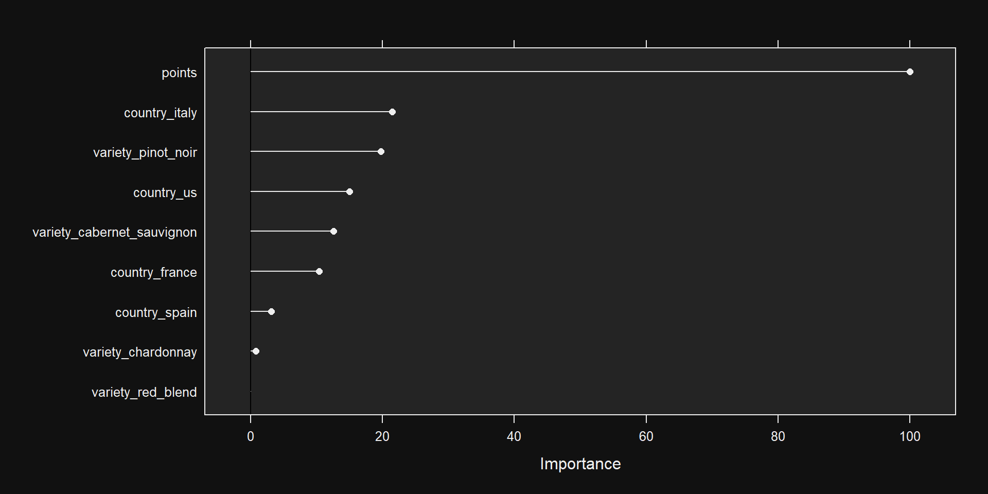
   points, country_us, country_italy, variety_cabernet_sauvignon, variety_pinot_noir

See Results

predictors(results)

[1] "points"                     "country_us"                
[3] "country_italy"              "variety_cabernet_sauvignon"
[5] "variety_pinot_noir"         "variety_red_blend"         
[7] "country_france"             "variety_chardonnay"        
[9] "country_spain"             

Plot Results

plot(results)

Practical Workflow

Key Terms

• Feature Engineering
• Categorical Feature
• Continuous Feature
• Dummy
• Interaction

• Caret
• Model
• Resampling
• Train vs. Test Data
• Variable Importance

Bonus Slides:
Linear Regression

5 Assumptions of Linear Regression

• Linear regressions have a well-developed statistical theory.

• This brings perks like confidence intervals on predictions.

• It also has “costs” in that assumptions need to be satisfied.

The Five

1. Linearity
2. Constant variance
3. Normality
4. Imperfect multicollinearity
5. Exogeneity

1. Linearity

• The dependent variable is a linear combination of the features.

• This is less of big deal than it might seem!

• If y is actually quadratic in x, then y is linear in x^2!

  • That’s feature engineering.

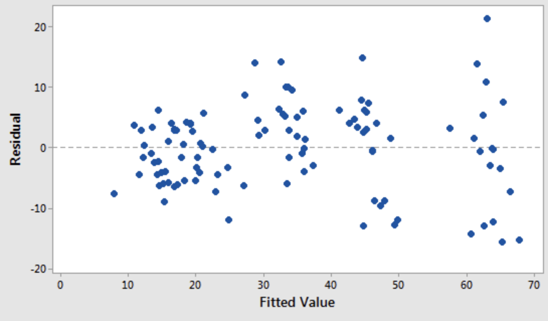
2. Constant variance

• Or homoscedasticity

• The variance of the errors do not depend on the values of the features.

• Don’t make bigger prediction errors for some values of x than for others.

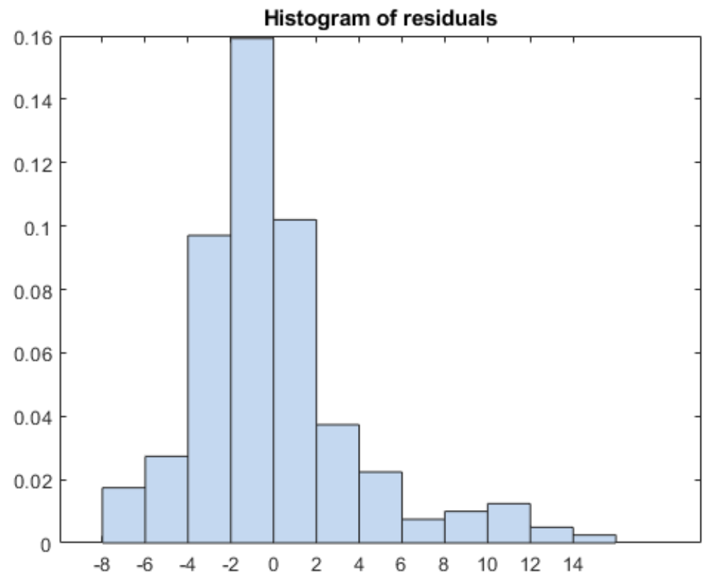
3. Normality

• The errors should be independent and normally distributed.

• A scatter plot of target variable value and residual (model error) should look like white noise.

4. Lack of perfect multicollinearity

• None predictors should be a perfect linear combination of others.

• This can happen if you over-engineer features

  • This is uncommon.
  • You’ll see an error that your coefficient matrix is singular or something.

5. Exogeneity

• Model errors should be independent of the values of the features.

• In particular, errors should have mean zero.

• It’s always good to look at a histogram of your residuals (see also normality).

First Test

• Determine whether the errors are normally distributed, like Shapiro-Wilk (also, plot them).

5 Assumptions of Linear Regression: testing

• Second I would always look at fitted value vs. residual to check homoscedasticity.

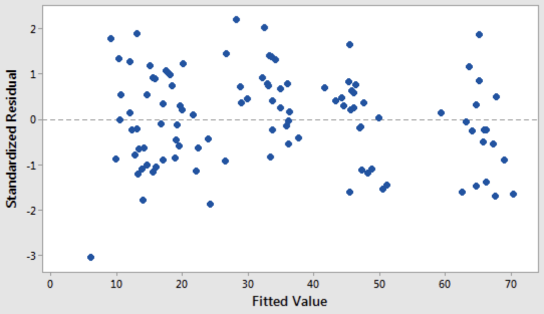
• For more, see for example https://people.duke.edu/~rnau/testing.htm