$K$ Nearest Neighbors

Applied Machine Learning

Jameson > Hendrik > Calvin

Agenda

Review of Homeworks
A human understanding of regression
Dinner break
Preprocessing and BoxCox
The $K$NN algorithm and the Confusion Matrix

Homework

HW1

We need to work on writing quality.
We need to work on RMSE intepretation.
We need to work on using summary responsibly.
We need to work on applying lecture topics to leading questions.
We would benefit from use of the embed-resources option in Quarto.

HW1 Sols Posted

Throwback ThMonday

I took my old grad ML repo down, but I’ve restored it.
Here
Takeaways:
- Everything is typeset.
  - Mathematics differentiated from
  - Code block differentiated from
  - Technical writing.
- No missing assets (e.g. images)
- Printable.

HW2

Think
Pair
Share

Today

Setup

library(tidyverse)
library(moderndive)
library(class)
library(caret)
library(fastDummies)
library(thematic)
theme_set(theme_dark())
thematic_rmd(bg = "#111", fg = "#eee", accent = "#eee")
wine <- readRDS(gzcon(url("https://cd-public.github.io/D505/dat/wine.rds"))) %>%
  mutate(lprice = log(price))

Reporting Impact from Regressions

Correlation

Credit: Modern Dive

http://guessthecorrelation.com/ …my high score is 72 (Jameson 122)

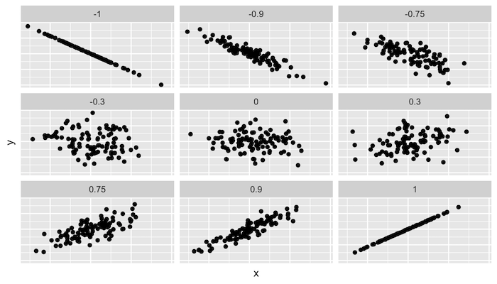
Calculating correlation

wine %>% 
  summarise(cor_p=cor(price,points),cor_lp=cor(lprice,points))

# A tibble: 1 × 2
  cor_p cor_lp
  <dbl>  <dbl>
1 0.404  0.624

Exercise

Calculate the correlation between $\log$(price) and points…
…by variety…
…for Oregon Chardonnay, Pinot Noir and Pinot Gris…
…in the same tibble!

Solution

wine %>% 
  filter(province=="Oregon") %>% 
  filter(variety %in% c("Chardonnay","Pinot Noir","Pinot Gris")) %>% 
  group_by(variety) %>% 
  summarise(correlation=cor(lprice,points))

# A tibble: 3 × 2
  variety    correlation
  <chr>            <dbl>
1 Chardonnay       0.642
2 Pinot Gris       0.490
3 Pinot Noir       0.591

Visualizing these different correlations

wine %>% 
  filter(province=="Oregon") %>% 
  filter(variety %in% c("Chardonnay","Pinot Noir","Pinot Gris")) %>% 
  ggplot(aes(points,lprice, color=variety)) +
    geom_point(alpha=0.3)+
    facet_wrap(~variety)+
    geom_smooth(method = lm)

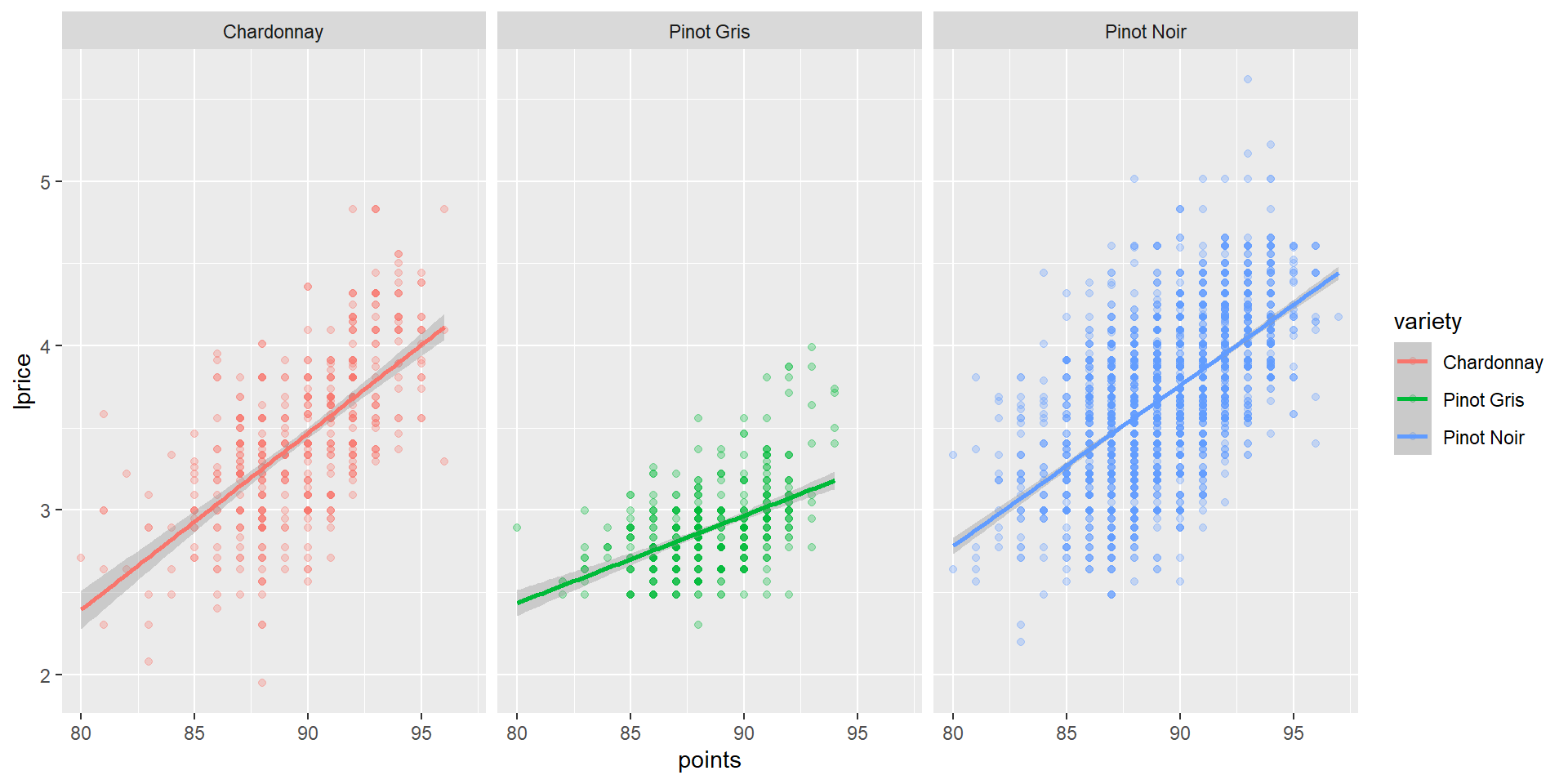
Visualizing these different correlations

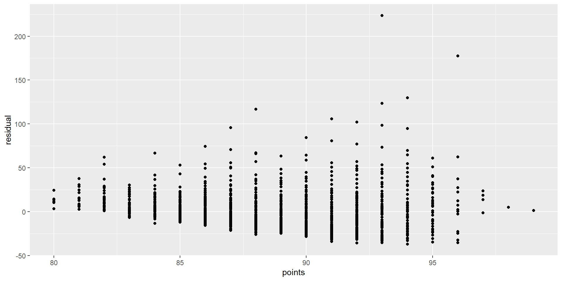
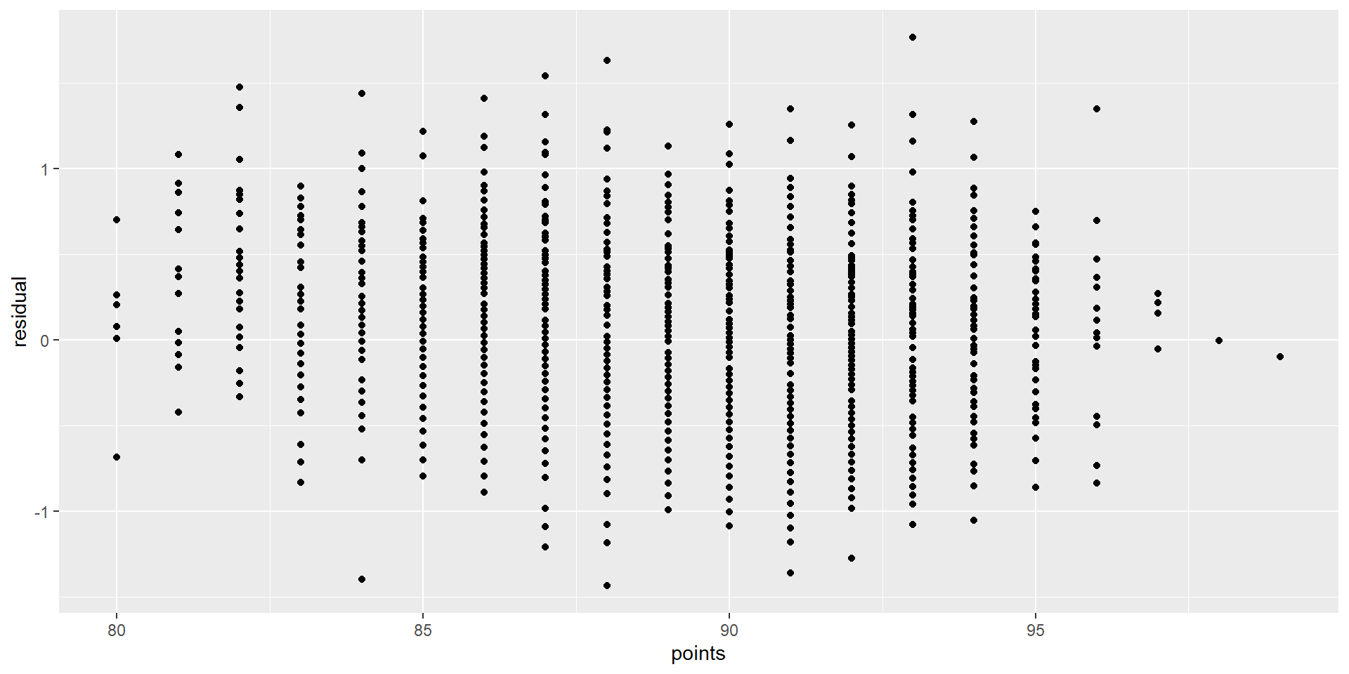
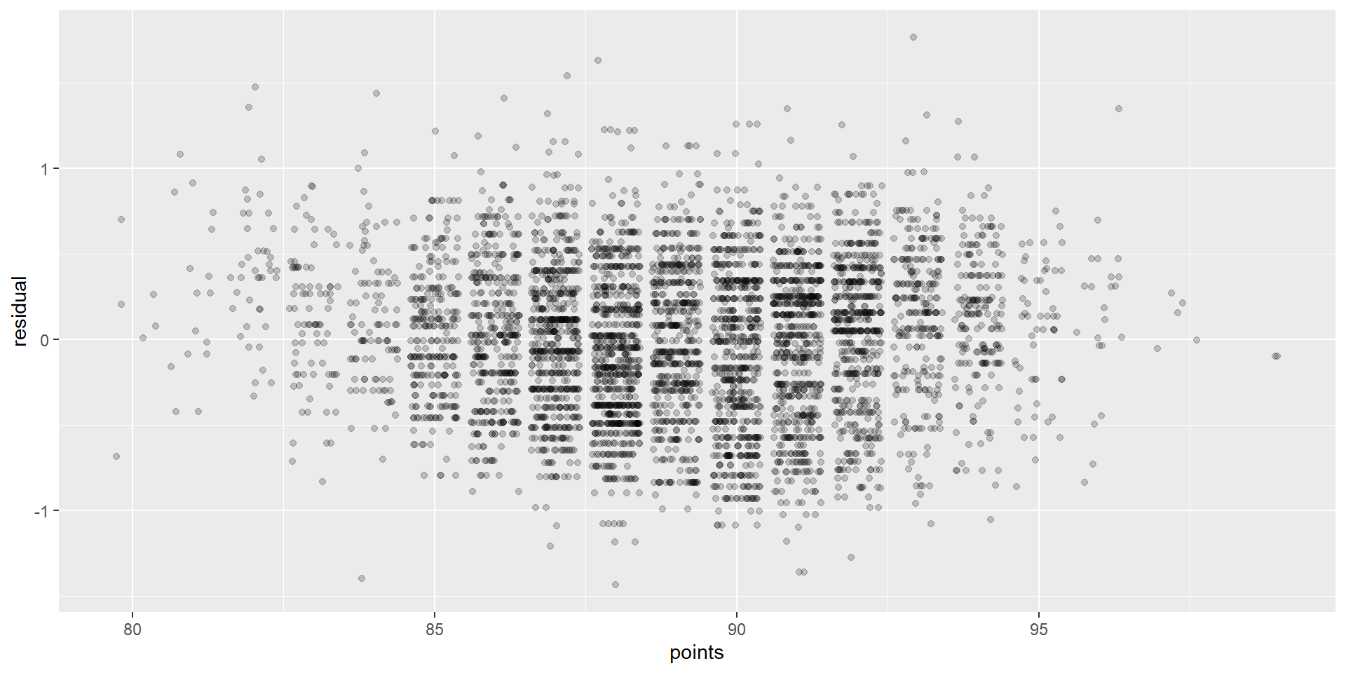
Graphing residuals (bad)

model <- lm(price~points, filter(wine,province=="Oregon"))
get_regression_points(model) %>% 
  ggplot(aes(points, residual))+
    geom_point()

Annotate

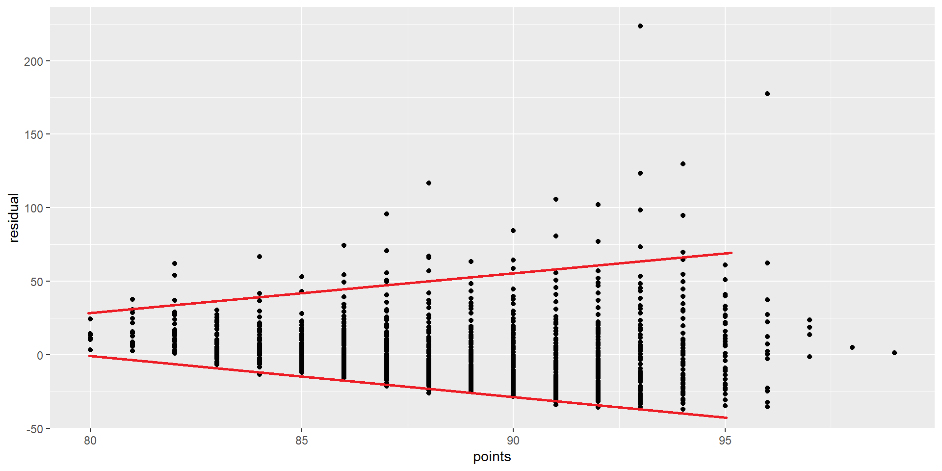
Graphing residuals (good)

model <- lm(lprice~points, filter(wine,province=="Oregon"))
get_regression_points(model) %>% 
  ggplot(aes(points, residual))+
    geom_point()

Interpreting the coefficients

model <- lm(lprice~points, filter(wine,province=="Oregon"))
pct = (exp(coef(model)["points"]) - 1) * 100
c(coef(model)["points"],pct)

    points     points 
0.09396111 9.85170227

We logged the dependent variable (price)
- A 1 point ratings increase = 9.85%
- That is, a percent change in rating to an absolute change in the dependent variable.
$(e^x - 1)*100$

Interpreting the coefficients

m_yr <- lm(lprice~year, filter(wine,province=="Oregon"))
yr = (exp(coef(m_yr)["year"]) - 1) * 100
c(coef(m_yr)["year"],yr)

      year       year 
0.01895092 1.91316309

This is a de facto measure of inflation.

Some Examples

for (x in 1:10) {
    print(c(x/100, (exp(x/100)-1) * 100))
}

[1] 0.010000 1.005017
[1] 0.020000 2.020134
[1] 0.030000 3.045453
[1] 0.040000 4.081077
[1] 0.05000 5.12711
[1] 0.060000 6.183655
[1] 0.070000 7.250818
[1] 0.080000 8.328707
[1] 0.090000 9.417428
[1]  0.10000 10.51709

for (x in 1:10) {
    print(c(x/010, (exp(x/010)-1) * 100))
}

[1]  0.10000 10.51709
[1]  0.20000 22.14028
[1]  0.30000 34.98588
[1]  0.40000 49.18247
[1]  0.50000 64.87213
[1]  0.60000 82.21188
[1]   0.7000 101.3753
[1]   0.8000 122.5541
[1]   0.9000 145.9603
[1]   1.0000 171.8282

Pretty Print

for(v in c("Chardonnay", "Pinot Gris","Pinot Noir")){
  m <- lm(lprice~points, filter(wine,province=="Oregon", variety==v))
  pct <- round((exp(coef(m)["points"]) - 1) * 100,2)
  print(str_c("For ",v,", a 1 point ratings increase leads to a ",pct,"% increase in price."))
}

[1] "For Chardonnay, a 1 point ratings increase leads to a 11.34% increase in price."
[1] "For Pinot Gris, a 1 point ratings increase leads to a 5.46% increase in price."
[1] "For Pinot Noir, a 1 point ratings increase leads to a 10.27% increase in price."

Summary

Only the dependent/response variable is log-transformed.
- Exponentiate the coefficient.
- Subtract one from this number
- Multiply by 100.
This gives the percent increase (or decrease).

$\log$ feature

model <- lm(price~lpoints, filter(wine,province=="Oregon") %>% mutate(lpoints=log(points)))
model


Call:
lm(formula = price ~ lpoints, data = filter(wine, province == 
    "Oregon") %>% mutate(lpoints = log(points)))

Coefficients:
(Intercept)      lpoints  
    -1419.0        324.4

What does the sign (positive or negative) tell us?
Was $\log$ appropriate here?

Percentages

coef(model)["lpoints"]/100

 lpoints 
3.243706

Since we logged the IV (feature), a 1% ratings increase is a ~3.24 increase in price on average.
What are the units on that?

Note: \[ x/100 \]

LogLog (also elasticity)

model <- lm(lprice~lpoints, filter(wine,province=="Oregon") %>% mutate(lpoints=log(points)))
model


Call:
lm(formula = lprice ~ lpoints, data = filter(wine, province == 
    "Oregon") %>% mutate(lpoints = log(points)))

Coefficients:
(Intercept)      lpoints  
    -33.770        8.298

…a 1% increase in ratings equals a 8.3% increase in price on average

Units

Change is per one-unit increase in the independent variable.
- Here, independent is points.
- Dependent is price.

Example

For every 1% increase in the independent variable…
- Basically, one point
- Our dependent variable increases by about 8.3%.
A $30 bottle of wine scoring 90 would be worth $32.50 as a 91.

30 * (1 + 8.3/100)

[1] 32.49

Graphing points by variety

wine %>% 
  filter(province=="Oregon") %>% 
  filter(variety %in% c("Chardonnay","Pinot Noir","Pinot Gris")) %>% 
  ggplot(aes(variety,points))+
    geom_boxplot()

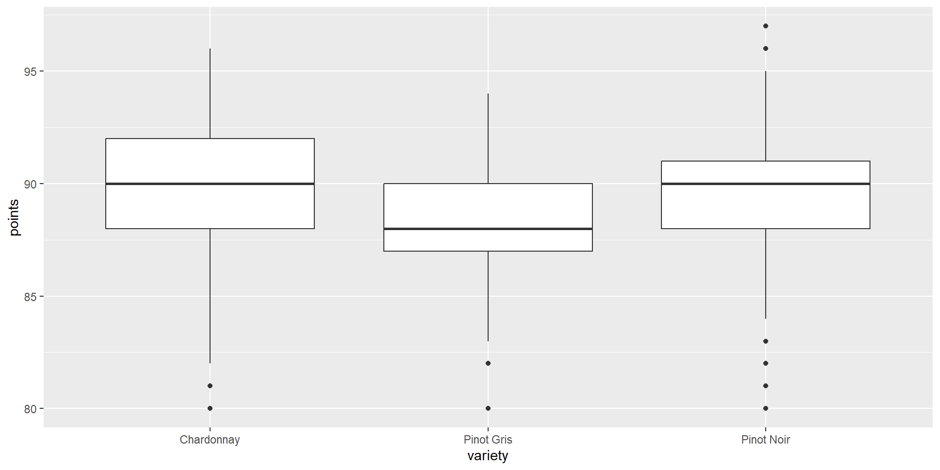
Summary

(tmp <- wine %>% 
  filter(province=="Oregon") %>% 
  filter(variety %in% c("Chardonnay","Pinot Noir","Pinot Gris")) %>% 
  group_by(variety) %>% 
  summarise(mean=mean(points)))

# A tibble: 3 × 2
  variety     mean
  <chr>      <dbl>
1 Chardonnay  89.7
2 Pinot Gris  88.5
3 Pinot Noir  89.5

What are the percentage differences here?

Regression

model <- lm(points~variety, 
            filter(wine,province=="Oregon",variety %in% c("Chardonnay","Pinot Noir","Pinot Gris")))
get_regression_table(model)

# A tibble: 3 × 7
  term                estimate std_error statistic p_value lower_ci upper_ci
  <chr>                  <dbl>     <dbl>     <dbl>   <dbl>    <dbl>    <dbl>
1 intercept             89.7       0.122    737.     0       89.5     90.0  
2 variety: Pinot Gris   -1.24      0.177     -7.03   0       -1.59    -0.894
3 variety: Pinot Noir   -0.256     0.132     -1.94   0.053   -0.515    0.003

What types of variables are we considering here?

Assumptions of linear regression

Linearity of relationship between variables
Independence of the residuals
Normality of the residuals
Equality of variance of the residuals

Linearity of relationship

Credit: Modern Dive

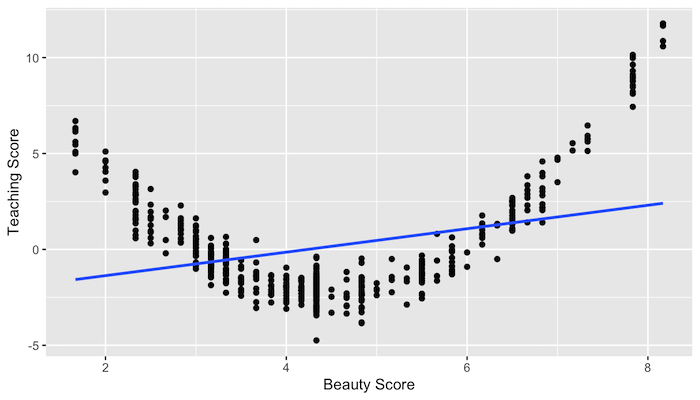
What would the residuals look like?

Independence

Given our original model of \[ \log(\text{price})=m*\text{Points}+b \]
are there any problems with independence?
How could we check?

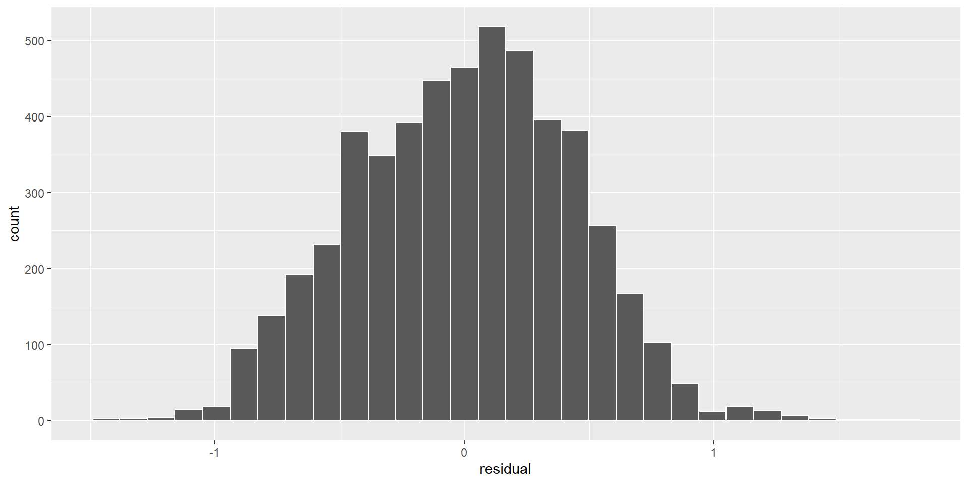
Normality

model <- lm(lprice~points, filter(wine,province=="Oregon"))
get_regression_points(model) %>% 
  ggplot(aes(residual))+
    geom_histogram(color="white")

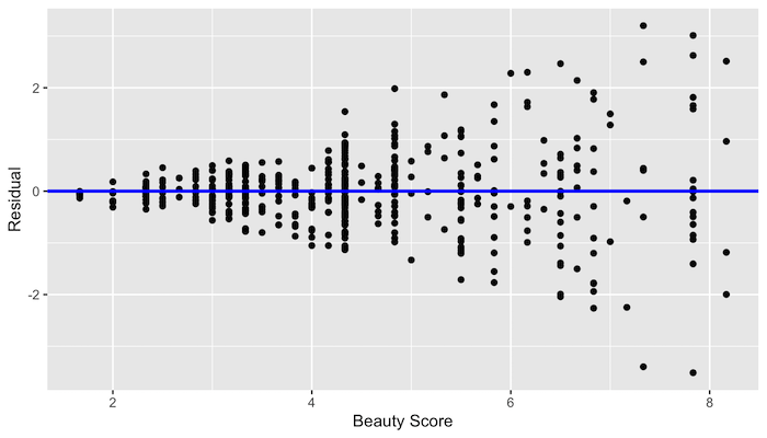
Equality of variance

get_regression_points(model) %>% 
  ggplot(aes(points, residual))+
    geom_jitter(alpha=0.2)

No equality in the variance

Credit: Modern Dive (click)

Dinner

Preprocessing and BoxCox

Setup

Pivot to pinot.
- Say “$\pi^0$”

wine <- readRDS(gzcon(url("https://cd-public.github.io/D505/dat/pinot_orig.rds")))

Preprocessing

Box-Cox transformations use maximum likelihood estimate to estimate value for $\lambda$

\[ y(\lambda) = \frac{x^{\lambda}-1}{\lambda} \]

The goal is to make data seem more like a normal distribution.

in R

LaTeX

\[ y(\lambda) = \frac{x^{\lambda}-1}{\lambda} \]

y <- function(A) {
  r <- function(x) {
    (x ** A - 1) / A
  }
}

Examples

When $\lambda=1$, there is no transformation

\[ y(1) = \frac{x^{\lambda}-1}{\lambda} = \frac{x^{1}-1}{1} = x-1 \approx x \]

\[ f = y(-1) \implies f(x) \approx x \]

Examples

When $\lambda=0$, it is log transformed

\[ y(0) = \frac{x^{\lambda}-1}{\lambda} = \frac{x^{0}-1}{0} \]

\[ f = y(0) \implies f(x) \approx \log(x) \]

Zero is a special case, but using a little thing called “calculus” this sorta makes sense.
Basically, negative infinity at 0, then increase slowly once positive.

$\lambda = 0$

for (x in 1:3) {
  print(x/10)
  for (l in 3:1) {
    f = y(l/100)
    print(c(l/100, x/10, f(x/10), log(x/10), f(x/10) - log(x/10)))
  }
}

[1] 0.1
[1]  0.03000000  0.10000000 -2.22485664 -2.30258509  0.07772845
[1]  0.02000000  0.10000000 -2.25037070 -2.30258509  0.05221439
[1]  0.01000000  0.10000000 -2.27627790 -2.30258509  0.02630719
[1] 0.2
[1]  0.0300000  0.2000000 -1.5712014 -1.6094379  0.0382365
[1]  0.0200000  0.2000000 -1.5838107 -1.6094379  0.0256272
[1]  0.01000000  0.20000000 -1.59655566 -1.60943791  0.01288225
[1] 0.3
[1]  0.03000000  0.30000000 -1.18248898 -1.20397280  0.02148382
[1]  0.02000000  0.30000000 -1.18959295 -1.20397280  0.01437985
[1]  0.010000000  0.300000000 -1.196754051 -1.203972804  0.007218753

Examples

\[ y(.5) = \frac{x^{\lambda}-1}{\lambda} = \frac{x^{.5}-1}{.5} = 2\times(\sqrt{x}-1) \approx \sqrt{x} \]

\[ f = y(.5) \implies f(x) \approx \sqrt{x} \]

Examples

When $\lambda=-1$, it is an inverse

\[ y(-1) = \frac{x^{\lambda}-1}{\lambda} = \frac{x^{-1}-1}{-1} = \frac{x^{-1}}{-1}+\frac{-1}{-1} = -x^{-1}-1 \approx x^{-1} \] \[ f = y(-1) \implies f(x) \approx x^{-1} \]

A Note

I am only aware of the following Box-Cox formulation:

\[ y(\lambda) = \begin{cases} \dfrac{y_i^\lambda - 1}{\lambda} & \text{if } \lambda \neq 0, \\ \ln y_i & \text{if } \lambda = 0, \end{cases} \]

Box-Cox is specified this way on Wikipedia, in Scikit documentation, in Scipy documentation.
I can only find one reference to $y(1)(x) \equiv x^{-1}$ here
- It’s citation are closed source.
There is no mention in the companion text ILSR

My Theory

This chart showed up in literature somewhere
Either a miscalculation or just some other transform.
It may be used in practice, including possibly in R?
It doesn’t matter they only change wrt scaled values.

-3	Y^-3 = 1/Y³
-2	Y^-2 = 1/Y²
-1	Y^-1 = 1/Y¹
-0.5	Y^-0.5 = 1/(√(Y))
0	log(Y)**
0.5	Y^0.5 = √(Y)
1	Y¹= Y
2	Y²
3	Y³

Just use the function

R: envstats

library(envstats)

# Example data
data <- c(1, 2, 3, 4, 5)

# Apply Box-Cox transformation
boxcox_result <- boxcoxTransform(data)

# Print the result
print(boxcox_result)

Just use the function

Py: scipy.stats

from scipy.stats import boxcox
import numpy as np

# Example data
data = np.array([1, 2, 3, 4, 5])

# Apply Box-Cox transformation
boxcox_result, lambda_value = boxcox(data)

# Print the result
print("Transformed data:", boxcox_result)
print("Lambda value:", lambda_value)

On Python

I like the Python boxcox documentation:

y = (x**lmbda - 1) / lmbda,  for lmbda != 0
    log(x),                  for lmbda = 0

This was how I tracked down what I believe to be the inconsistency with other Box-Cox definitions.

Onward

Caret preprocessing is so easy!

wine %>% 
  preProcess(method = c("BoxCox","center","scale")) %>% 
  predict(wine) %>% 
  select(-description) %>% 
  head()

    province      price    points        year    taster_name
1     Oregon  0.7146905 -1.033841 -0.03425331   Paul Gregutt
2     Oregon -1.4139991 -1.033841  0.33313680   Paul Gregutt
3 California  0.8225454 -1.033841 -0.40146088 Virginie Boone
4     Oregon  0.2408520 -1.367723 -0.76848588   Paul Gregutt
5     Oregon -1.2418658 -1.367723 -1.13532834   Paul Gregutt
6     Oregon -1.0109945 -1.367723  1.06846470   Paul Gregutt

Or is it?

But wait… what is wrong here?

wino <- wine %>%
  mutate(year_f = as.factor(year))

wino <- wino %>% 
  preProcess(method = c("BoxCox","center","scale")) %>% 
  predict(wino)

head(wino %>% select(starts_with("year")))

         year year_f
1 -0.03425331   2012
2  0.33313680   2013
3 -0.40146088   2011
4 -0.76848588   2010
5 -1.13532834   2009
6  1.06846470   2015

Are years normally distributed?

The $K$NN Algorithm

Algorithm

Load the data
Initialize $K$ to your chosen number of neighbors
For each example in the data

Calculate the distance between the query example and the current example from the data.
Add the distance and the index of the example to an ordered collection

Sort the ordered collection of distances and indices from smallest to largest (in ascending order) by the distances
Pick the first $K$ entries from the sorted collection
Get the labels of the selected $K$ entries
If regression, return the mean of the $K$ labels
If classification, return the mode of the $K$ labels

Basis

We assume:
- Existing datapoints in something we think of as a space
  - That is, probably two numerical value per point in a coordinate plane
  - Categorical is fine - think a Punnett square
- Existing datapoints are labelled
  - Numerical or categorical still fine!
To visualize, we will have a 2d space with color labels.

Let’s draw it

Let’s draw it 2

Let’s draw it 3

G4G

Engineering some features

Create an “other” for most tasters.

wino <- wino %>% 
  mutate(taster_name = fct_lump(taster_name,5))

Engineering some features

Create dummys for years, tasters

wino <- wino %>% dummy_cols(
    select_columns = c("year_f","taster_name"),
    remove_most_frequent_dummy = T, 
    remove_selected_columns = T)

Engineering some features

Convert everything to snake case.

wino <- wino %>% 
  rename_all(funs(tolower(.))) %>% 
  rename_all(funs(str_replace_all(., "-", "_"))) %>% 
  rename_all(funs(str_replace_all(., " ", "_")))

Engineering some features

Add indicators for 3 tasting notes.

wino <- wino %>% 
  mutate(note_cherry = str_detect(description,"cherry")) %>% 
  mutate(note_chocolate = str_detect(description,"chocolate")) %>%
  mutate(note_earth = str_detect(description,"earth")) %>%
  select(-description)

Engineering some features

Let’s see it

head(wino) %>% 
  select(1:6)

    province      price    points        year year_f_1996 year_f_1997
1     Oregon  0.7146905 -1.033841 -0.03425331           0           0
2     Oregon -1.4139991 -1.033841  0.33313680           0           0
3 California  0.8225454 -1.033841 -0.40146088           0           0
4     Oregon  0.2408520 -1.367723 -0.76848588           0           0
5     Oregon -1.2418658 -1.367723 -1.13532834           0           0
6     Oregon -1.0109945 -1.367723  1.06846470           0           0

Split

set.seed(505)
wine_index <- createDataPartition(wino$province, p = 0.8, list = FALSE)
train <- wino[ wine_index, ]
test <- wino[-wine_index, ]

Simple model

Specify a $K$NN model.

fit <- knn(
  train = select(train,-province), 
  test = select(test,-province), 
  k=5, 
  cl = train$province)

Confusion matrix

Let’s look at Kappa.

confusionMatrix(fit,factor(test$province))$overall

      Accuracy          Kappa  AccuracyLower  AccuracyUpper   AccuracyNull 
     0.9360430      0.9012588      0.9232355      0.9472929      0.4728033 
AccuracyPValue  McnemarPValue 
     0.0000000            NaN

Kappa $\kappa$ statistic

Kappa statistic is a measurement of the agreement for categorical items Kappa can be used to assess the performance of kNN algorithm.

\[ \kappa = \dfrac{P(A)-P(E)}{1 - P(E)} \]

where $P(A)$ is the relative observed agreement among raters, and $P(E)$ is the proportion of agreement expected between the classifier and the ground truth by chance.

Kappa $\kappa$ statistic

Rule of thumb.

< 0.2 (not so good)
0.21 - 0.4 (ok)
0.41 - 0.6 (pretty good)
0.6 - 0.8 (great)
> 0.8 (almost perfect)

We had ~.9…

Overfitting… or a leak?

Review the dataframe

summary(wino)

   province             price              points               year        
 Length:8380        Min.   :-3.31001   Min.   :-3.289952   Min.   :-5.8877  
 Class :character   1st Qu.:-0.62250   1st Qu.:-0.696100   1st Qu.:-0.4015  
 Mode  :character   Median : 0.05057   Median :-0.009039   Median : 0.3331  
                    Mean   : 0.00000   Mean   : 0.000000   Mean   : 0.0000  
                    3rd Qu.: 0.57013   3rd Qu.: 0.693463   3rd Qu.: 0.7007  
                    Max.   : 7.30609   Max.   : 2.893605   Max.   : 1.0685  
  year_f_1996         year_f_1997         year_f_1998        year_f_1999      
 Min.   :0.0000000   Min.   :0.0000000   Min.   :0.000000   Min.   :0.000000  
 1st Qu.:0.0000000   1st Qu.:0.0000000   1st Qu.:0.000000   1st Qu.:0.000000  
 Median :0.0000000   Median :0.0000000   Median :0.000000   Median :0.000000  
 Mean   :0.0001193   Mean   :0.0002387   Mean   :0.008353   Mean   :0.002029  
 3rd Qu.:0.0000000   3rd Qu.:0.0000000   3rd Qu.:0.000000   3rd Qu.:0.000000  
 Max.   :1.0000000   Max.   :1.0000000   Max.   :1.000000   Max.   :1.000000  
  year_f_2000        year_f_2001        year_f_2002        year_f_2003       
 Min.   :0.000000   Min.   :0.000000   Min.   :0.000000   Min.   :0.0000000  
 1st Qu.:0.000000   1st Qu.:0.000000   1st Qu.:0.000000   1st Qu.:0.0000000  
 Median :0.000000   Median :0.000000   Median :0.000000   Median :0.0000000  
 Mean   :0.001074   Mean   :0.000358   Mean   :0.000358   Mean   :0.0001193  
 3rd Qu.:0.000000   3rd Qu.:0.000000   3rd Qu.:0.000000   3rd Qu.:0.0000000  
 Max.   :1.000000   Max.   :1.000000   Max.   :1.000000   Max.   :1.0000000  
  year_f_2004        year_f_2005       year_f_2006       year_f_2007     
 Min.   :0.000000   Min.   :0.00000   Min.   :0.00000   Min.   :0.00000  
 1st Qu.:0.000000   1st Qu.:0.00000   1st Qu.:0.00000   1st Qu.:0.00000  
 Median :0.000000   Median :0.00000   Median :0.00000   Median :0.00000  
 Mean   :0.002029   Mean   :0.01539   Mean   :0.01957   Mean   :0.01432  
 3rd Qu.:0.000000   3rd Qu.:0.00000   3rd Qu.:0.00000   3rd Qu.:0.00000  
 Max.   :1.000000   Max.   :1.00000   Max.   :1.00000   Max.   :1.00000  
  year_f_2008       year_f_2009       year_f_2010      year_f_2011     
 Min.   :0.00000   Min.   :0.00000   Min.   :0.0000   Min.   :0.00000  
 1st Qu.:0.00000   1st Qu.:0.00000   1st Qu.:0.0000   1st Qu.:0.00000  
 Median :0.00000   Median :0.00000   Median :0.0000   Median :0.00000  
 Mean   :0.02733   Mean   :0.04129   Mean   :0.0599   Mean   :0.06945  
 3rd Qu.:0.00000   3rd Qu.:0.00000   3rd Qu.:0.0000   3rd Qu.:0.00000  
 Max.   :1.00000   Max.   :1.00000   Max.   :1.0000   Max.   :1.00000  
  year_f_2012      year_f_2013      year_f_2015      taster_name_jim_gordon
 Min.   :0.0000   Min.   :0.0000   Min.   :0.00000   Min.   :0.00000       
 1st Qu.:0.0000   1st Qu.:0.0000   1st Qu.:0.00000   1st Qu.:0.00000       
 Median :0.0000   Median :0.0000   Median :0.00000   Median :0.00000       
 Mean   :0.1796   Mean   :0.2171   Mean   :0.09726   Mean   :0.06563       
 3rd Qu.:0.0000   3rd Qu.:0.0000   3rd Qu.:0.00000   3rd Qu.:0.00000       
 Max.   :1.0000   Max.   :1.0000   Max.   :1.00000   Max.   :1.00000       
 taster_name_matt_kettmann taster_name_other taster_name_roger_voss
 Min.   :0.0000            Min.   :0.00000   Min.   :0.0000        
 1st Qu.:0.0000            1st Qu.:0.00000   1st Qu.:0.0000        
 Median :0.0000            Median :0.00000   Median :0.0000        
 Mean   :0.1826            Mean   :0.06993   Mean   :0.1415        
 3rd Qu.:0.0000            3rd Qu.:0.00000   3rd Qu.:0.0000        
 Max.   :1.0000            Max.   :1.00000   Max.   :1.0000        
 taster_name_virginie_boone note_cherry     note_chocolate  note_earth     
 Min.   :0.0000             Mode :logical   Mode :logical   Mode :logical  
 1st Qu.:0.0000             FALSE:5017      FALSE:7830      FALSE:7030     
 Median :0.0000             TRUE :3363      TRUE :550       TRUE :1350     
 Mean   :0.2223                                                            
 3rd Qu.:0.0000                                                            
 Max.   :1.0000

Determine what dominates

omit <- function(prefix) {
  train <- select(train, -starts_with(prefix))
  test <- select(test, -starts_with(prefix))
  fit <- knn(
    train = select(train,-province), 
    test = select(test,-province), 
    k=5, 
    cl = train$province)
  confusionMatrix(fit,factor(test$province))$overall
}

Test

c(omit('year')["Kappa"], omit('note')["Kappa"], omit('taster')["Kappa"])

    Kappa     Kappa     Kappa 
0.9318353 0.9280857 0.3523416

Fixing the leak

Dastardly humans, always existing in a physical location.

train <- select(train, -starts_with("taster"))
test <- select(test, -starts_with("taster"))

Rerun

fit <- knn(
  train = select(train,-province), 
  test = select(test,-province), 
  k=5, 
  cl = train$province)

We should probably have written function here!
That is a lot of lines to copy+paste…

Confusion matrix

confusionMatrix(fit,factor(test$province))

Confusion Matrix and Statistics

                   Reference
Prediction          Burgundy California Casablanca_Valley Marlborough New_York
  Burgundy               120         42                 4           8        3
  California              51        582                 9          14        5
  Casablanca_Valley        2          1                 0           0        2
  Marlborough              1          5                 2           5        4
  New_York                 0          3                 3           2        3
  Oregon                  64        158                 8          16        9
                   Reference
Prediction          Oregon
  Burgundy              58
  California           201
  Casablanca_Valley      1
  Marlborough           11
  New_York               3
  Oregon               273

Overall Statistics
                                          
               Accuracy : 0.5876          
                 95% CI : (0.5635, 0.6113)
    No Information Rate : 0.4728          
    P-Value [Acc > NIR] : < 2.2e-16       
                                          
                  Kappa : 0.348           
                                          
 Mcnemar's Test P-Value : 0.0006799       

Statistics by Class:

                     Class: Burgundy Class: California Class: Casablanca_Valley
Sensitivity                  0.50420            0.7358                 0.000000
Specificity                  0.91986            0.6825                 0.996357
Pos Pred Value               0.51064            0.6752                 0.000000
Neg Pred Value               0.91794            0.7423                 0.984403
Prevalence                   0.14226            0.4728                 0.015541
Detection Rate               0.07173            0.3479                 0.000000
Detection Prevalence         0.14047            0.5152                 0.003586
Balanced Accuracy            0.71203            0.7092                 0.498179
                     Class: Marlborough Class: New_York Class: Oregon
Sensitivity                    0.111111        0.115385        0.4991
Specificity                    0.985872        0.993321        0.7735
Pos Pred Value                 0.178571        0.214286        0.5170
Neg Pred Value                 0.975684        0.986136        0.7607
Prevalence                     0.026898        0.015541        0.3270
Detection Rate                 0.002989        0.001793        0.1632
Detection Prevalence           0.016736        0.008368        0.3156
Balanced Accuracy              0.548492        0.554353        0.6363

With parameter tuning over $K$

fit <- train(province ~ .,
             data = train, 
             method = "knn",
             tuneLength = 15,
             trControl = trainControl(number = 1)) # default bootstrap
fit

k-Nearest Neighbors 

6707 samples
  25 predictor
   6 classes: 'Burgundy', 'California', 'Casablanca_Valley', 'Marlborough', 'New_York', 'Oregon' 

No pre-processing
Resampling: Bootstrapped (1 reps) 
Summary of sample sizes: 6707 
Resampling results across tuning parameters:

  k   Accuracy   Kappa    
   5  0.5585216  0.3107902
   7  0.5626283  0.3107703
   9  0.5663244  0.3130763
  11  0.5860370  0.3396248
  13  0.5905544  0.3456984
  15  0.5909651  0.3423630
  17  0.5938398  0.3434720
  19  0.5991786  0.3493659
  21  0.6016427  0.3516418
  23  0.5995893  0.3472121
  25  0.6049281  0.3556879
  27  0.6028747  0.3507932
  29  0.6032854  0.3504058
  31  0.6016427  0.3467558
  33  0.6049281  0.3510662

Accuracy was used to select the optimal model using the largest value.
The final value used for the model was k = 33.

Confusion Matrix

confusionMatrix(predict(fit, test),factor(test$province))

Confusion Matrix and Statistics

                   Reference
Prediction          Burgundy California Casablanca_Valley Marlborough New_York
  Burgundy               109         24                 4           7        1
  California              72        682                10          16        9
  Casablanca_Valley        0          0                 0           0        0
  Marlborough              1          0                 2           2        1
  New_York                 1          0                 1           0        1
  Oregon                  55         85                 9          20       14
                   Reference
Prediction          Oregon
  Burgundy              44
  California           248
  Casablanca_Valley      1
  Marlborough            2
  New_York               0
  Oregon               252

Overall Statistics
                                          
               Accuracy : 0.6252          
                 95% CI : (0.6015, 0.6485)
    No Information Rate : 0.4728          
    P-Value [Acc > NIR] : < 2.2e-16       
                                          
                  Kappa : 0.3812          
                                          
 Mcnemar's Test P-Value : < 2.2e-16       

Statistics by Class:

                     Class: Burgundy Class: California Class: Casablanca_Valley
Sensitivity                  0.45798            0.8622                0.0000000
Specificity                  0.94425            0.5975                0.9993928
Pos Pred Value               0.57672            0.6577                0.0000000
Neg Pred Value               0.91307            0.8286                0.9844498
Prevalence                   0.14226            0.4728                0.0155409
Detection Rate               0.06515            0.4077                0.0000000
Detection Prevalence         0.11297            0.6198                0.0005977
Balanced Accuracy            0.70112            0.7299                0.4996964
                     Class: Marlborough Class: New_York Class: Oregon
Sensitivity                    0.044444       0.0384615        0.4607
Specificity                    0.996314       0.9987857        0.8375
Pos Pred Value                 0.250000       0.3333333        0.5793
Neg Pred Value                 0.974174       0.9850299        0.7617
Prevalence                     0.026898       0.0155409        0.3270
Detection Rate                 0.001195       0.0005977        0.1506
Detection Prevalence           0.004782       0.0017932        0.2600
Balanced Accuracy              0.520379       0.5186236        0.6491

Tuning and subsampling

fit <- train(province ~ .,
             data = train, 
             method = "knn",
             tuneLength = 15,
             metric = "Kappa", # this is new
             trControl = trainControl(number = 1))
fit

k-Nearest Neighbors 

6707 samples
  25 predictor
   6 classes: 'Burgundy', 'California', 'Casablanca_Valley', 'Marlborough', 'New_York', 'Oregon' 

No pre-processing
Resampling: Bootstrapped (1 reps) 
Summary of sample sizes: 6707 
Resampling results across tuning parameters:

  k   Accuracy   Kappa    
   5  0.5662211  0.3335443
   7  0.5897124  0.3626746
   9  0.5953827  0.3643307
  11  0.6022681  0.3694469
  13  0.6083435  0.3735947
  15  0.6051033  0.3662155
  17  0.6030782  0.3598731
  19  0.6006480  0.3528698
  21  0.6083435  0.3635047
  23  0.6127987  0.3709898
  25  0.6119887  0.3672124
  27  0.6132037  0.3679552
  29  0.6103686  0.3629132
  31  0.6091535  0.3605970
  33  0.6103686  0.3619960

Kappa was used to select the optimal model using the largest value.
The final value used for the model was k = 13.

Tuning plot

ggplot(fit, metric="Kappa")

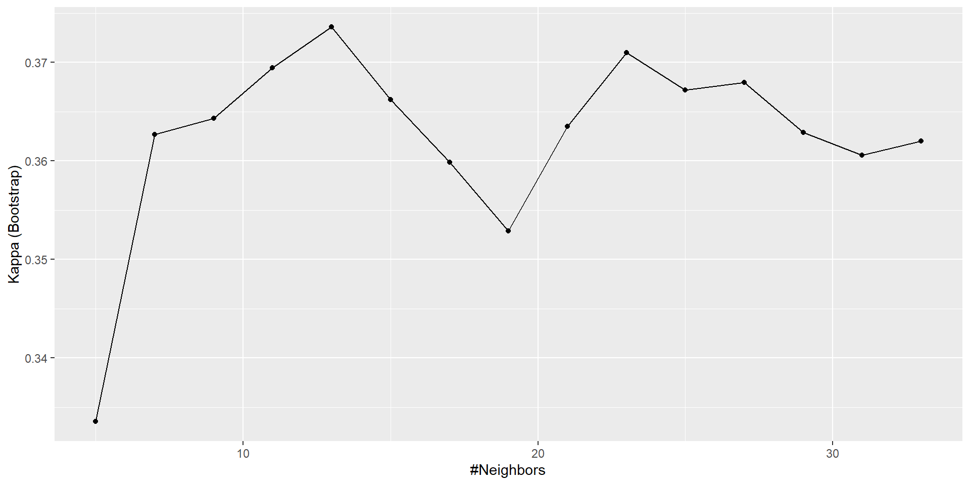
Group modeling problem I

Practice running different versions of the model
Create some new features and…
See if you can achieve a Kappa >= 0.5!

\[ \kappa \geq 0.5 \]

Bonus: KNN for regression

fit <- train(price ~ .,
             data = train, 
             method = "knn",
             tuneLength = 15,
             trControl = trainControl(number = 1))
fit

k-Nearest Neighbors 

6707 samples
  25 predictor

No pre-processing
Resampling: Bootstrapped (1 reps) 
Summary of sample sizes: 6707 
Resampling results across tuning parameters:

  k   RMSE       Rsquared   MAE      
   5  0.7088713  0.4838682  0.5496792
   7  0.7068384  0.4844876  0.5477807
   9  0.7079209  0.4825940  0.5503138
  11  0.7120092  0.4761552  0.5526014
  13  0.7099825  0.4789842  0.5511644
  15  0.7066122  0.4840501  0.5494917
  17  0.7029911  0.4897134  0.5463464
  19  0.7045467  0.4880710  0.5475400
  21  0.7034253  0.4902028  0.5467853
  23  0.7040237  0.4907806  0.5467905
  25  0.7026135  0.4933143  0.5458847
  27  0.7020678  0.4946617  0.5452430
  29  0.7039476  0.4932789  0.5455563
  31  0.7066255  0.4905195  0.5467215
  33  0.7063276  0.4918182  0.5480512

RMSE was used to select the optimal model using the smallest value.
The final value used for the model was k = 27.

\(K\) Nearest Neighbors

Agenda

Homework

HW1

HW1 Sols Posted

Throwback ThMonday

HW2

Today

Setup

Reporting Impact from Regressions

Correlation

Calculating correlation

Exercise

Solution

Visualizing these different correlations

Visualizing these different correlations

Graphing residuals (bad)

Annotate

Graphing residuals (good)

Interpreting the coefficients

Interpreting the coefficients

Some Examples

Pretty Print

Summary

\(\log\) feature

Percentages

LogLog (also elasticity)

Units

Example

Graphing points by variety

Summary

Regression

Assumptions of linear regression

Linearity of relationship

Independence

Normality

Equality of variance

No equality in the variance

Dinner

Preprocessing and BoxCox

Setup

Preprocessing

in R

Examples

Examples

\(\lambda = 0\)

Examples

Examples

A Note

My Theory

Just use the function

Just use the function

On Python

Onward

Caret preprocessing is so easy!

Or is it?

The \(K\)NN Algorithm

Algorithm

Basis

Let’s draw it

Let’s draw it 2

Let’s draw it 3

Engineering some features

Engineering some features

Engineering some features

Engineering some features

Engineering some features

Split

Simple model

Confusion matrix

Kappa \(\kappa\) statistic

Kappa \(\kappa\) statistic

Overfitting… or a leak?

Review the dataframe

Determine what dominates

Test

Fixing the leak

Rerun

Confusion matrix

With parameter tuning over \(K\)