[1] 0.52000000 0.04807692Naive Bayes
Applied Machine Learning
Jameson > Hendrik > Calvin
Agenda
- Group Prep Work
- Homework
- The Naive Bayes algorithm
- Tidy text and bag of words
- Group work
- Vocabulary
Groups
Modeling Dates
- Mar 10
- Mar 17
- Apr 28
Group Preference Form
- Fill this out.
- Full link:
Homework
HW3
- Think
- Pair
- Share
The Naive Bayes Algorithm
Shorter
\[ P(c|x) = \frac{P(x|c)P(c)}{P(x)} = \frac{P(c \space \land \space x)}{P(x)} \]
- Take \(\land\) to be “logical and”
- The probability of both
candx, basically.
Longer
\[ P(L~|~{\rm features}) = \frac{P({\rm features}~|~L)P(L)}{P({\rm features})} \]
- More generally…
\[ P({\rm A}~|~{\rm B}) = \frac{P({\rm B}~|~ \rm{A})P(\rm{A})}{P({\rm B})} \]
Bayes’ Theorem Example
- Suppose
- Half of all emails are spam
- You’ve just purchased some software (hurray) that filters spam emails
- It claims to detect 99% of spam
- It claims the probability of a false positive (marking non-spam as spam) is 5%.
Bayes’ Theorem Example
- “Suppose half of all emails are spam…””
P(is_spam) = .5
- “detect 99% of spam”
P(called_spam|is_spam) = .99
- “(marking non-spam as spam) is 5%”
P(called_spam|isnt_spam) = .5
Bayes’ Theorem Example
- Now suppose an incoming email is marked as spam. What is the probability that it’s a non-spam email?
- \(A\) = email is non-spam email
- \(B\) = email is marked as spam
- P(\(B\) | \(A\)) =
- P(\(A\)) =
- P(\(B\)) =
Bayes’ Theorem Example Solution
- \(A\) = email is non-spam email = .5
- \(B\) = email is marked as spam = ??
- P(\(B\) | \(A\)) = .05
- P(\(A\)) = .5
- P(\(B\)) = .99 * .5 + .05 * .5
- P(\(A\) | \(B\)) = .05 * .5 / (.99 * .5 + .05 * .5)
Exercise 1
- You have three cards:
- one is red on both sides,
- one is black on both sides, and
- one has one red side and one black side.
- You pick a card at random, and
- put it on the table on a random side, and
- the color showing is red.
- What is the probability that the other side is black?
Solution 1
- \(A\) = card is red-black = 1/3
- \(B\) = side up is red = ??
- P(\(B\) | \(A\)) == 1/2
- P(\(B\)) = 1 * 1/3 + 1/2 * 1/3 + 0 * 1/3 = 1.5/3 = 1/2
- P(\(A\) | \(B\)) = 1/3 * 1/2 / (1/2) = 1/3
Exercise 2
- Imagine half of all rainy days start off cloudy in the morning.
- However, we live in a cloudy place, and…
- about 40% of days start off cloudy, and…
- 90% of days this time of year do not have rain.
- What are the odds it will rain today?
Solution 2
- \(A\) = rain during the day = .1
- \(B\) = cloudy in the morning = .4
- P(\(B\) | \(A\)) = .5
- P(\(A\) | \(B\)) = 0.1*0.5 / 0.4 = 0.125
Algorithm
\[ P({\rm Cherry}~|~{\rm Chardonnay}) * P({\rm Fruit}~|~{\rm Chardonnay}) * P({\rm Bordeaux}~|~{\rm Chardonnay}) \]
- Choosing between two labels \(L_1\) and \(L_2\):
\[ \frac{P(L_1~|~{\rm features})}{P(L_2~|~{\rm features})} = \frac{P({\rm features}~|~L_1)}{P({\rm features}~|~L_2)}\frac{P(L_1)}{P(L_2)} \]
Uh oh
- But how on earth can we get \(P({\rm features}~|~L)\)$?
- Well, we have to make an assumption.
- “Naive” in Naive Bayes means we keep it simple.
Example
- Really we would need P(Cherry, Fruit, Bordeaux | Chardonnay)
- “Naive” assumption is independence so the algorithm calculates:
\[ \begin{align} P({\rm Cherry} &~|~ {\rm Chardonnay}) *\\ P({\rm Fruit} &~|~ {\rm Chardonnay}) *\\ P({\rm Bordeaux} &~|~ {\rm Chardonnay}) \end{align} \]
Setup
library(tidyverse)
library(caret)
library(fastDummies)
library(thematic)
library(naivebayes) # New
library(tidytext) # New
theme_set(theme_dark())
thematic_rmd(bg = "#111", fg = "#eee", accent = "#eee")
wine <- readRDS(gzcon(url("https://cd-public.github.io/D505/dat/pinot.rds")))
names(wine)[names(wine) == 'id'] = 'ID'
Some basic features
wino <- wine %>%
  mutate(year_f = as.factor(year)) %>%
  mutate(cherry = str_detect(description,"cherry")) %>%
  mutate(chocolate = str_detect(description,"chocolate")) %>%
  mutate(earth = str_detect(description,"earth")) %>%
  select(-description, year)

glimpse(wino)
Rows: 8,380
Columns: 9
$ ID <int> 1, 2, 3, 4, 5, 6, 7, 8, 9, 10, 11, 12, 13, 14, 15, 16, 17, 1…
$ province <chr> "Oregon", "Oregon", "California", "Oregon", "Oregon", "Orego…
$ price <dbl> 65, 20, 69, 50, 22, 25, 64, 55, 44, 38, 28, 45, 22, 55, 40, …
$ points <dbl> 87, 87, 87, 86, 86, 86, 91, 91, 91, 91, 85, 85, 85, 89, 89, …
$ year <dbl> 2012, 2013, 2011, 2010, 2009, 2015, 2013, 2012, 2014, 2014, …
$ year_f <fct> 2012, 2013, 2011, 2010, 2009, 2015, 2013, 2012, 2014, 2014, …
$ cherry <lgl> FALSE, FALSE, FALSE, FALSE, FALSE, FALSE, FALSE, TRUE, FALSE…
$ chocolate <lgl> FALSE, TRUE, FALSE, FALSE, FALSE, FALSE, FALSE, FALSE, FALSE…
$ earth <lgl> TRUE, FALSE, TRUE, FALSE, TRUE, FALSE, FALSE, FALSE, FALSE, …Conditional probability
\(p(Oregon | cherry) = \frac{p(Oregon \space\&\space Cherry)}{p(Cherry)}\)
How about New York?
\(p(NY | cherry) = \frac{p(NY \space\&\space Cherry)}{p(Cherry)}\)
A basic model
A basic model
Naive Bayes

6707 samples
   8 predictor
   6 classes: 'Burgundy', 'California', 'Casablanca_Valley', 'Marlborough', 'New_York', 'Oregon'

No pre-processing
Resampling: Cross-Validated (10 fold)
Summary of sample sizes: 6037, 6037, 6036, 6036, 6036, 6037, ...
Resampling results across tuning parameters:

  usekernel  Accuracy   Kappa
  FALSE      0.4792050  0.17112459
   TRUE      0.3553707  0.03408878

Tuning parameter 'laplace' was held constant at a value of 0
Tuning
 parameter 'adjust' was held constant at a value of 1
Kappa was used to select the optimal model using the largest value.
The final values used for the model were laplace = 0, usekernel = FALSE
 and adjust = 1.
Maybe bin the data?
wino <- wino %>%
  select(-starts_with("year_")) %>%
  mutate(points_f = case_when(
    points < 90 ~ "low",
    points >= 90 & points < 96 ~ "med",
    points >= 96 ~ "high"
  )
           )  %>%
  mutate(price_f = case_when(
    price < 16 ~ "low",
    price >= 16 & price < 41 ~ "med",
    price >= 41 ~ "high"
  )
           )  %>%
  mutate(year_f = case_when(
    year < 2005 ~ "old",
    year >= 2005 & year < 2011 ~ "recent",
    year >= 2011 ~ "current"
  )
           ) %>%
  select(-price,-points,-year)

head(wino)
Maybe bin the data?
  ID   province cherry chocolate earth points_f price_f  year_f
1  1     Oregon  FALSE     FALSE  TRUE      low    high current
2  2     Oregon  FALSE      TRUE FALSE      low     med current
3  3 California  FALSE     FALSE  TRUE      low    high current
4  4     Oregon  FALSE     FALSE FALSE      low    high  recent
5  5     Oregon  FALSE     FALSE  TRUE      low     med  recent
6  6     Oregon  FALSE     FALSE FALSE      low     med current
Binned model
Binned model
Naive Bayes

6707 samples
   7 predictor
   6 classes: 'Burgundy', 'California', 'Casablanca_Valley', 'Marlborough', 'New_York', 'Oregon'

No pre-processing
Resampling: Cross-Validated (10 fold)
Summary of sample sizes: 6036, 6034, 6036, 6038, 6034, 6038, ...
Resampling results across tuning parameters:

  usekernel  Accuracy   Kappa
  FALSE      0.4544189  0.2545278
   TRUE      0.5206607  0.1511061

Tuning parameter 'laplace' was held constant at a value of 0
Tuning
 parameter 'adjust' was held constant at a value of 1
Kappa was used to select the optimal model using the largest value.
The final values used for the model were laplace = 0, usekernel = FALSE
 and adjust = 1.
Confusion Matrix
Confusion Matrix and Statistics

                   Reference
Prediction          Burgundy California Casablanca_Valley Marlborough New_York
  Burgundy               208        308                10          20        6
  California              19        421                 2          10       10
  Casablanca_Valley        2         23                10           4        3
  Marlborough              0          3                 1           1        1
  New_York                 1          5                 1           7        5
  Oregon                   8         31                 2           3        1
                   Reference
Prediction          Oregon
  Burgundy             269
  California           140
  Casablanca_Valley      8
  Marlborough           10
  New_York              11
  Oregon               109

Overall Statistics

               Accuracy : 0.4507
                 95% CI : (0.4267, 0.4749)
    No Information Rate : 0.4728
    P-Value [Acc > NIR] : 0.9669

                  Kappa : 0.2464

 Mcnemar's Test P-Value : <2e-16

Statistics by Class:

                     Class: Burgundy Class: California Class: Casablanca_Valley
Sensitivity                   0.8739            0.5322                 0.384615
Specificity                   0.5728            0.7948                 0.975713
Pos Pred Value                0.2533            0.6993                 0.200000
Neg Pred Value                0.9648            0.6545                 0.990142
Prevalence                    0.1423            0.4728                 0.015541
Detection Rate                0.1243            0.2516                 0.005977
Detection Prevalence          0.4907            0.3598                 0.029886
Balanced Accuracy             0.7234            0.6635                 0.680164
                     Class: Marlborough Class: New_York Class: Oregon
Sensitivity                   0.0222222        0.192308       0.19927
Specificity                   0.9907862        0.984821       0.96004
Pos Pred Value                0.0625000        0.166667       0.70779
Neg Pred Value                0.9734460        0.987219       0.71165
Prevalence                    0.0268978        0.015541       0.32696
Detection Rate                0.0005977        0.002989       0.06515
Detection Prevalence          0.0095637        0.017932       0.09205
Balanced Accuracy             0.5065042        0.588564       0.57965
Tidytext and frequency distributions
Tidytext
Stop Words
Example
Matrix
- We adopt the convention of refering to our dataframe as “df”
- Short for
drofessor falvin
  ID   province price points year
1  1     Oregon    65     87 2012
2  2     Oregon    20     87 2013
3  3 California    69     87 2011
4  4     Oregon    50     86 2010
5  5     Oregon    22     86 2009
6  6     Oregon    25     86 2015
                                                                                                                                                                                                                                                                                       description
1                                        Much like the regular bottling from 2012, this comes across as rather rough and tannic, with rustic, earthy, herbal characteristics. Nonetheless, if you think of it as a pleasantly unfussy country wine, it's a good companion to a hearty winter stew.
2                                                        A sleek mix of tart berry, stem and herb, along with a hint of oak and chocolate, this is a fair value in a widely available, drink-now Oregon Pinot. The wine oak-aged for six months, whether in neutral or re-staved is not indicated.
3                              Oak and earth intermingle around robust aromas of wet forest floor in this vineyard-designated Pinot that hails from a high-elevation site. Small in production, it offers intense, full-bodied raspberry and blackberry steeped in smoky spice and smooth texture.
4                                               As with many of the Erath 2010 vineyard designates, this is strongly herbal. The notes of leaf and herb create somewhat unripe flavor impressions, with a touch of bitterness on the finish. The fruit just passes the ripeness of sweet tomatoes.
5                                                                                                                              A stiff, tannic wine, this slowly opens and brings brambly berry flavors into play, along with notes of earthy herbs. There's a touch of bitterness to the tannins.
6 Some rosés are made simply by bleeding the juice from the fermenter, to concentrate the remaining wine. Whether or not that is the case here, the wine has the simple pleasant lightly candied strawberry flavors one might expect from such a technique. It's fruity and undemanding. Drink up.- We’ll build it incrementally and check-in as we go.
Bird Up
- With apologies to Eric Andre
- We really just want words, don’t need them in like sentences or whatever.
Grammy Snub
- Anti (2016) was snubbed don’t @ me
- Remove “boring” words
\(\pi^0\)
- Won’t see much visible change here.
- But including these could cook our data.
Id, Ego, Superego
- We left in IDs like 3 hours ago.
- Use them to aggregate words.
Group Ease
- With words attached to IDs…
- We can structure into a wine compatibile dataframe
Big Ole Freq
- Just like Megan’s first charting song…
- Most words occur once
\(\exists\)
- Make sure words occur AT ALL
- \(\forall {\rm words} \exists {\rm ID }\)
Individualism
- Words were grouped up by ID
- Pool them back together.
Transpose
- Group on words now that frequencies are found for ids.
Accumulate
- At long last, we have a description as some numerical data type.
# A tibble: 6 × 6
# Groups:   word [6]
     ID word                n   freq exists total
  <int> <chr>           <int>  <dbl> <lgl>  <int>
1     1 2012                1 0.0588 TRUE      71
2     1 bottling            1 0.0588 TRUE     849
3     1 characteristics     1 0.0588 TRUE      61
4     1 companion           1 0.0588 TRUE      22
5     1 country             1 0.0588 TRUE      11
6     1 earthy              1 0.0588 TRUE     804
Results
- We essential have words by popularity.
Join
- Have you seen
LEFT JOINin 503 yet? - W3
The LEFT JOIN keyword returns all records from the left table (table1), and the matching records from the right table (table2). The result is 0 records from the right side, if there is no match.- G4G
In SQL, LEFT JOIN retrieves all records from the left table and only the matching records from the right table. When there is no matching record found, NULL values are returned for columns from the right table. This makes LEFT JOIN extremely useful for queries where you need to retain all records from one table, even if there is no corresponding match in the other table.IDs
- Keep your ID around…
- We are so back.
# A tibble: 6 × 7
# Groups:   word [6]
     ID word                n   freq exists total province
  <int> <chr>           <int>  <dbl> <lgl>  <int> <chr>
1     1 2012                1 0.0588 TRUE      71 Oregon
2     1 bottling            1 0.0588 TRUE     849 Oregon
3     1 characteristics     1 0.0588 TRUE      61 Oregon
4     1 companion           1 0.0588 TRUE      22 Oregon
5     1 country             1 0.0588 TRUE      11 Oregon
6     1 earthy              1 0.0588 TRUE     804 Oregon
Use those words!
df %>%
  count(province, word) %>%
  group_by(province) %>%
  top_n(5,n) %>%
  arrange(province, desc(n)) %>%
  head()
# A tibble: 6 × 3
# Groups: province [2]
word province n
<chr> <chr> <int>
1 tannins Burgundy 763
2 drink Burgundy 673
3 acidity Burgundy 652
4 red Burgundy 630
5 fruits Burgundy 575
6 cherry California 1917Group exercise
Use the top words by province to…
- Engineer more features that capture the essence of Casablanca, Marlborough and New York
- Look for difference between California and Oregon
- Use what you find to run naive Bayes models that achieve a Kappa that approaches 0.5
Vocabulary
- Naive Bayes
- Correlation
- Residual
- Kappa
- Parameter Tuning
- Conditional Probability
Stinger
library(scales)
wtxt <- wine %>%
unnest_tokens(word, description) %>%
anti_join(stop_words) %>%
filter(str_detect(string = word, pattern = "[a-z+]")) %>% # get rid weird non alphas
filter(str_length(word)>3) %>% # get rid of strings shorter than 3 characters
group_by(word) %>%
mutate(total=n()) %>%
ungroup()
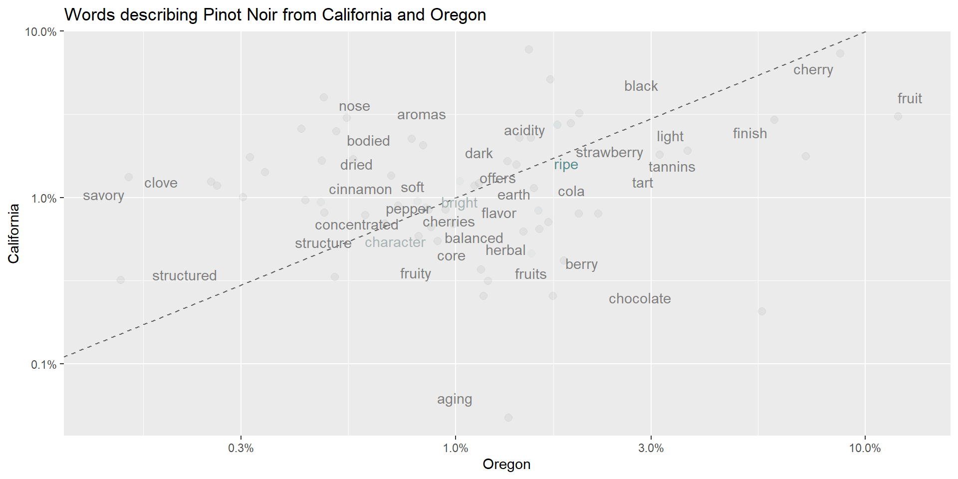
wtxt %>%
filter(province=="Oregon" | province=="California") %>%
filter(!(word %in% c("wine","pinot","drink","noir","vineyard","palate","notes","flavors","bottling"))) %>%
filter(total > 400) %>%
group_by(province, word) %>%
count() %>%
group_by(province) %>%
mutate(proportion = n / sum(n)) %>%
pivot_wider(id_cols = word, names_from = province, values_from = proportion) %>%
ggplot(aes(x = Oregon, y = California, color = abs(Oregon - California))) +
geom_abline(color = "gray40", lty = 2) +
geom_jitter(alpha = 0.1, size = 2.5, width = 0.3, height = 0.3) +
geom_text(aes(label = word), check_overlap = TRUE, vjust = 1.5) +
scale_x_log10(labels = percent_format()) +
scale_y_log10(labels = percent_format()) +
scale_color_gradient(limits = c(0, 0.001), low = "darkslategray4", high = "gray75") +
theme(legend.position="none") +
labs(x = "Oregon", y = "California", title = "Words describing Pinot Noir from California and Oregon")Stinger
Stinger
dtxt <- wtxt %>%
filter(province=="Oregon" | province=="California") %>%
filter(!(word %in% c("wine","pinot","drink","noir","vineyard","palate","notes","flavors","bottling","bottle","finish"))) %>%
filter(total > 400) %>%
group_by(province, word) %>%
count() %>%
group_by(province) %>%
mutate(proportion = n / sum(n)) %>%
pivot_wider(id_cols = word, names_from = province, values_from = proportion) %>%
mutate(diff=Oregon-California)
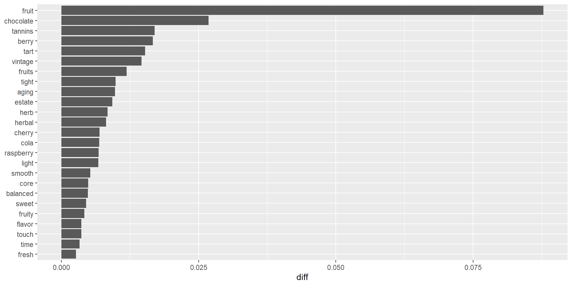
dtxt %>%
top_n(25, diff) %>%
mutate(word = reorder(word, diff)) %>%
ggplot(aes(word, diff)) +
geom_col() +
xlab(NULL) +
coord_flip()Stinger