Logistic Regression

Applied Machine Learning

Jameson > Calvin

Agenda

Course Announcements
Mathematics of logistic regression
Implementation with Caret
ROC Curves
Group work

Midterm 3/17

Brief recap of course so far

Linear regression (e.g. lprice ~ .), assumptions of model, interpretation.
\(K\)-NN (e.g., province ~ .), multi-class supervised classification. Hyperparameter \(k\).
Naive Bayes (e.g., province ~ .), multi-class supervised classification.
Logistic regression (e.g., province=="Oregon" ~ .), binary supervised classification. Elastic net.
Feature engineering (logarithms, center/scaling, Box Cox, tidytext, etc.).
Feature selection (correlation, linear / logistic coefficients, frequent words, frequent words by class, etc.).

Practice

I am working to develop a practice midterm.
I will circulate it by 3 Mar.
You will go over it on 10 Mar.
It is based on the 5 homeworks.
It is based on the prior slide.
- Little to no computatational linguistics
- I’m regarding tidytext as extension, not core, content.

Modality Discussion

I would release an assignment electronically at 6 PM
We can do in person or otherwise.
It will be “cheat proof”
- I will ask you nothing for which it matters how you determine the answer.
- If e.g. ChatGPT can be mind controlled into doing high quality feature engineering, you get points for mind controlling ChatGPT.

First Model Due 3/10

Publish

Each group should create: 1. An annotated .*md file, and 2. The .rds/.pickle/.parquet file that it generates, that 3. Contains only the features you want in the model.

Under version control, on GitHub.

Constraints

I will run:

The specified \(K\)NN or Naive Bayes model,
With: province ~ . (or the whole data frame in scikit)
With repeated 5-fold cross validation
With the same index for partitioning training and test sets for every group.
On whatever is turned in before class.
Bragging rights for highest Kappa

Context

The “final exam” is that during the last class you will present your model results as though you are speaking to the managers of a large winery.
It should be presented from a Quarto presentation on GitHub or perhaps e.g. RPubs.
You must present via the in-room “teaching machine” computer, not your own physical device, to ensure that you are comfortable distributing your findings.

Group Meetings

You should have a group assignment
Meet in your groups!
Talk about your homework with your group.

Logistic Regression

Algorithm

Assume a linear relationship between the log odds and a set of predictor variables.

\[ log(\frac{p}{1-p})=\beta_{0}+\beta_{1}x_{1}+\beta_{2}x_{2} \]

With a bit of algebra you can get the probabilities as…

\[ p=\frac{1}{1+e^{-(\beta_{0}+\beta_{1}x_{1}+\beta_{2}x_{2})}} \]

\[ log(\frac{p}{1-p})=\beta_{0}+\beta_{1}x_{1}+\beta_{2}x_{2} \]

‘p’ represents the probability of the event occurring.

Represented as natural log ln…
of the odds ratio (\(\frac{p}{1-p}\))…
as a linear combination of
- predictor variables (\(x_1\), \(x_2\)) and
- their corresponding coefficients (\(\beta_1\), \(\beta_2\))
- plus an intercept (\(\beta_0\)).

Understanding check?

Why do we call this regression instead of classification?
Quick Algebra review
- Look, it’s better to be comfortable with algebra than not.

Log Odds

1. Start with the log-odds equation:

\[ log(\frac{p}{1-p}) = \beta_0 + \beta_1x_1 + \beta_2x_2 \]

Exponentiate

2. Exponentiate both sides:
To remove the logarithm, we take the exponential (e) of both sides of the equation:

\[ e^{log(\frac{p}{1-p})} = e^{\beta_0 + \beta_1x_1 + \beta_2x_2} \]

Simplify

3. Simplify the left side:
The exponential function and the natural logarithm are inverse functions of each other.
Therefore, \(e^{log(x)} = x\). This simplifies the left side:

\[ \frac{p}{1-p} = e^{\beta_0 + \beta_1x_1 + \beta_2x_2} \]

Rewrite

4. Rewrite the right side using exponent rules:
We can rewrite the right side using the rule \(e^{a+b} = e^a * e^b\):

\[ \frac{p}{1-p} = e^{\beta_0} * e^{\beta_1x_1} * e^{\beta_2x_2} \]

Find \(p\) 1

1. Find \(p\)
- Multiply both sides by (1-p):

\[ p = (1-p) * e^{\beta_0} * e^{\beta_1x_1} * e^{\beta_2x_2} \]

Find \(p\) 2

1. Find \(p\)
- Distribute the right-hand side (RHS):

\[ p = e^{\beta_0} * e^{\beta_1x_1} * e^{\beta_2x_2} - p * e^{\beta_0} * e^{\beta_1x_1} * e^{\beta_2x_2} \]

Find \(p\) 2

1. Find \(p\)
- Move the \(p\) term to the left side:

\[ p + p * e^{\beta_0} * e^{\beta_1x_1} * e^{\beta_2x_2} = e^{\beta_0} * e^{\beta_1x_1} * e^{\beta_2x_2} \]

Find \(p\) 3

1. Find \(p\)
- Factor out \(p\) on the left side:

\[ p * (1 + e^{\beta_0} * e^{\beta_1x_1} * e^{\beta_2x_2}) = e^{\beta_0} * e^{\beta_1x_1} * e^{\beta_2x_2} \]

Find \(p\) 4

1. Find \(p\)
- Divide both sides by the term in parentheses: \[ p = \frac{e^{\beta_0} * e^{\beta_1x_1} * e^{\beta_2x_2}}{1 + e^{\beta_0} * e^{\beta_1x_1} * e^{\beta_2x_2}} \]

Simplify

6. Simplify the expression:
We can further simplify by multiplying the numerator and denominator by \(e^{-(\beta_0 + \beta_1x_1 + \beta_2x_2)}\):

\[ p = \frac{1}{e^{-(\beta_0 + \beta_1x_1 + \beta_2x_2)} + 1} \]

Rewrite

Which is commonly written as:

\[ p = \frac{1}{1 + e^{-(\beta_0 + \beta_1x_1 + \beta_2x_2)}} \]

Implementation with Caret

Libraries Setup

sh <- suppressPackageStartupMessages
sh(library(tidyverse))
sh(library(caret))
sh(library(tidytext))
sh(library(SnowballC)) # new?
sh(library(pROC))      # new?
sh(library(glmnet))
data(stop_words)
sh(library(thematic))
theme_set(theme_dark())
thematic_rmd(bg = "#111", fg = "#eee", accent = "#eee")

Dataframe

wine <- readRDS(gzcon(url("https://cd-public.github.io/D505/dat/pinot.rds")))
names(wine)[names(wine) == 'id'] = 'id'

Extract certain words

We’ll proceed in a few steps.
- First, a function to extract all words.
  - We’ll omit stopwords
    - Remember those? Like “of” and “a”
  - We’ll omit a few words-of-choice
    - Like “pinot”

Extract all words

desc_to_words <- function(df, omits) { 
  df %>%
    unnest_tokens(word, description) %>%
    anti_join(stop_words) %>% # get rid of stop words
    filter(!(word %in% omits))
}

Extract all words

words <- desc_to_words(wine, c("wine","pinot","vineyard"))
# The second argument is our custom stopwards, as a vector
head(words)

  id province price points year     word
1  1   Oregon    65     87 2012  regular
2  1   Oregon    65     87 2012 bottling
3  1   Oregon    65     87 2012     2012
4  1   Oregon    65     87 2012    rough
5  1   Oregon    65     87 2012   tannic
6  1   Oregon    65     87 2012   rustic

Extract certain words

We’ll proceed in a few steps.
- Optionally, look at stems
  - This is really cool.
  - Do I care about the difference between “acidic” and “acidity”?
    - The linguistics consensus leans toward no.

STEM

Short for data Science, daTa science, data sciencE, and Machine learning.

words_to_stems <- function(df) { 
  df %>%
    mutate(word = wordStem(word))
}

We want to use a tidytext built-in here, of course.
- We aren’t domain experts in linguistics…
- But we are domain experts in using R libraries.

Example

Stem may either consist of a root (e.g. run) alone or a compound word, such as meatball and bottleneck (examples of compound nouns) or blacken and standardize (examples of compound verbs). The stem of the verb to wait is wait: it is the part that is common to all its inflected variants.

Wait

‘wait’ (infinitive, imperative, present subjunctive, and present indicative except in the 3rd-person singular)
‘waits’ (3rd person singular simple present indicative)
‘waited’ (simple past)
‘waited’ (past participle)
‘waiting’ (present participle)

STEM

stems <- words_to_stems(words)
head(stems)

  id province price points year    word
1  1   Oregon    65     87 2012 regular
2  1   Oregon    65     87 2012   bottl
3  1   Oregon    65     87 2012    2012
4  1   Oregon    65     87 2012   rough
5  1   Oregon    65     87 2012  tannic
6  1   Oregon    65     87 2012  rustic

Bottl

Another example.

g6_df <- tibble(description = "Popping bottles in the ice; like a blizzard.")
words_to_stems(desc_to_words(g6_df, c("ice")))

# A tibble: 3 × 1
  word    
  <chr>   
1 pop     
2 bottl   
3 blizzard

Like a G6

Word Count

With either or words or our stems, we can see how many of each word we have easily enough.
- And eliminate words will less than a certain count!

filter_by_count <- function(df, j) { 
  df %>%
    count(id, word) %>% 
    group_by(id) %>% mutate(exists = (n>0)) %>% ungroup %>% 
    group_by(word) %>% 
    mutate(total = sum(n)) %>% 
    filter(total > j)
}

Check it

fwords = filter_by_count(words, 1000)
head(fwords)

# A tibble: 6 × 5
# Groups:   word [5]
     id word          n exists total
  <int> <chr>     <int> <lgl>  <int>
1     2 drink         1 TRUE    1388
2     2 oak           2 TRUE    1198
3     3 aromas        1 TRUE    1459
4     3 bodied        1 TRUE    1016
5     3 oak           1 TRUE    1198
6     3 raspberry     1 TRUE    1394

fstems = filter_by_count(stems, 1000)
head(fstems)

# A tibble: 6 × 5
# Groups:   word [6]
     id word      n exists total
  <int> <chr> <int> <lgl>  <int>
1     1 bottl     1 TRUE    1229
2     2 ag        1 TRUE    1101
3     2 berri     1 TRUE    1028
4     2 drink     1 TRUE    1573
5     2 oak       2 TRUE    1225
6     3 aroma     1 TRUE    1601

Back to Wine

We currently have multiple entries per ID in a tidy dataframe
We would like to get back to have features for each ID, as each ID is some wine.
One way to do so, is to make columns from the word data.
We use pivot_wider

Pivot

pivoter <- function(words, df) {
  words %>%
    pivot_wider(id_cols = id, names_from = word, values_from = exists, values_fill = list(exists=0)) %>% 
    right_join(select(df,id,province)) %>% 
    drop_na() %>% 
    select(-id)
}

Check it

head(pivoter(fwords, wine))

# A tibble: 6 × 23
  drink oak   aromas bodied raspberry spice finish fruit flavors tannins
  <lgl> <lgl> <lgl>  <lgl>  <lgl>     <lgl> <lgl>  <lgl> <lgl>   <lgl>  
1 TRUE  TRUE  FALSE  FALSE  FALSE     FALSE FALSE  FALSE FALSE   FALSE  
2 FALSE TRUE  TRUE   TRUE   TRUE      TRUE  FALSE  FALSE FALSE   FALSE  
3 FALSE FALSE FALSE  FALSE  FALSE     FALSE TRUE   TRUE  FALSE   FALSE  
4 FALSE FALSE FALSE  FALSE  FALSE     FALSE FALSE  FALSE TRUE    TRUE   
5 TRUE  FALSE FALSE  FALSE  FALSE     FALSE FALSE  FALSE TRUE    FALSE  
6 FALSE FALSE FALSE  FALSE  TRUE      FALSE FALSE  FALSE FALSE   FALSE  
# ℹ 13 more variables: strawberry <lgl>, cranberry <lgl>, dark <lgl>,
#   palate <lgl>, acidity <lgl>, black <lgl>, cherry <lgl>, nose <lgl>,
#   ripe <lgl>, light <lgl>, red <lgl>, plum <lgl>, province <chr>

head(pivoter(fstems, wine))

# A tibble: 6 × 30
  bottl ag    berri drink oak   aroma bodi  offer raspberri spice textur finish
  <lgl> <lgl> <lgl> <lgl> <lgl> <lgl> <lgl> <lgl> <lgl>     <lgl> <lgl>  <lgl> 
1 TRUE  FALSE FALSE FALSE FALSE FALSE FALSE FALSE FALSE     FALSE FALSE  FALSE 
2 FALSE TRUE  TRUE  TRUE  TRUE  FALSE FALSE FALSE FALSE     FALSE FALSE  FALSE 
3 FALSE FALSE FALSE FALSE TRUE  TRUE  TRUE  TRUE  TRUE      TRUE  TRUE   FALSE 
4 FALSE FALSE FALSE FALSE FALSE FALSE FALSE FALSE FALSE     FALSE FALSE  TRUE  
5 FALSE FALSE TRUE  FALSE FALSE FALSE FALSE FALSE FALSE     FALSE FALSE  FALSE 
6 FALSE FALSE FALSE TRUE  FALSE FALSE FALSE FALSE FALSE     FALSE FALSE  FALSE 
# ℹ 18 more variables: flavor <lgl>, fruit <lgl>, ripe <lgl>, tannin <lgl>,
#   strawberri <lgl>, cranberri <lgl>, dark <lgl>, palat <lgl>, acid <lgl>,
#   black <lgl>, cherri <lgl>, nose <lgl>, light <lgl>, red <lgl>, rich <lgl>,
#   plum <lgl>, structur <lgl>, province <chr>

Full Function

Create a function to extract words with totals > j

wine_words <- function(df, j, stem) { 

  words <- desc_to_words(df, c("wine","pinot","vineyard"))
  
  if (stem) {
    words <- words_to_stems(words)
  }
  
  words <- filter_by_count(words, j)

  pivoter(words, df)
}

Look at the data

wino <- wine_words(wine, 1000, F)

wino %>% 
  head(10) %>% 
  select(1:5, province)

# A tibble: 10 × 6
   drink oak   aromas bodied raspberry province  
   <lgl> <lgl> <lgl>  <lgl>  <lgl>     <chr>     
 1 TRUE  TRUE  FALSE  FALSE  FALSE     Oregon    
 2 FALSE TRUE  TRUE   TRUE   TRUE      California
 3 FALSE FALSE FALSE  FALSE  FALSE     Oregon    
 4 FALSE FALSE FALSE  FALSE  FALSE     Oregon    
 5 TRUE  FALSE FALSE  FALSE  FALSE     Oregon    
 6 FALSE FALSE FALSE  FALSE  TRUE      California
 7 FALSE FALSE FALSE  FALSE  TRUE      California
 8 FALSE TRUE  FALSE  FALSE  TRUE      California
 9 FALSE FALSE FALSE  FALSE  FALSE     Oregon    
10 FALSE FALSE TRUE   FALSE  FALSE     Oregon

Logistic Regression

We check a true/false outcome.

wino <- wino %>% 
  mutate(oregon = factor(province=="Oregon")) %>%
  select(-province)

wino %>% 
  head(10) %>% 
  select(1:5, oregon)

# A tibble: 10 × 6
   drink oak   aromas bodied raspberry oregon
   <lgl> <lgl> <lgl>  <lgl>  <lgl>     <fct> 
 1 TRUE  TRUE  FALSE  FALSE  FALSE     TRUE  
 2 FALSE TRUE  TRUE   TRUE   TRUE      FALSE 
 3 FALSE FALSE FALSE  FALSE  FALSE     TRUE  
 4 FALSE FALSE FALSE  FALSE  FALSE     TRUE  
 5 TRUE  FALSE FALSE  FALSE  FALSE     TRUE  
 6 FALSE FALSE FALSE  FALSE  TRUE      FALSE 
 7 FALSE FALSE FALSE  FALSE  TRUE      FALSE 
 8 FALSE TRUE  FALSE  FALSE  TRUE      FALSE 
 9 FALSE FALSE FALSE  FALSE  FALSE     TRUE  
10 FALSE FALSE TRUE   FALSE  FALSE     TRUE

Split the data

wine_index <- createDataPartition(wino$oregon, p = 0.80, list = FALSE)
train <- wino[ wine_index, ]
test <- wino[-wine_index, ]
table(train$oregon)


FALSE  TRUE 
 4487  2156

A basic model

control = trainControl(method = "cv", number = 5)
get_fit <- function(df) {
  train(oregon ~ .,
        data = df, 
        trControl = control,
        method = "glm",
        family = "binomial",
        maxit = 5) # speed it up - default 100
}
fit <- get_fit(train)

Check Kappa

fit

Penalized Multinomial Regression 

6644 samples
  22 predictor
   6 classes: 'Burgundy', 'California', 'Casablanca_Valley', 'Marlborough', 'New_York', 'Oregon' 

No pre-processing
Resampling: Cross-Validated (5 fold) 
Summary of sample sizes: 5315, 5315, 5315, 5316, 5315 
Resampling results across tuning parameters:

  decay  Accuracy   Kappa    
  0e+00  0.7245610  0.5683360
  1e-04  0.7245610  0.5683360
  1e-01  0.7251632  0.5691676

Accuracy was used to select the optimal model using the largest value.
The final value used for the model was decay = 0.1.

Probability

See top coefficients

get_odds <- function(fit) {
  as.data.frame(t(exp(coef(fit$finalModel))))   %>%
  rownames_to_column(var = "name") %>%
  pivot_longer(-name, names_to = "class", values_to = "odds") %>%
  arrange(desc(odds)) %>%
  head()
}
get_odds(fit)

# A tibble: 6 × 3
  name        class              odds
  <chr>       <chr>             <dbl>
1 bodiedTRUE  California         5.19
2 (Intercept) Oregon             3.92
3 noseTRUE    California         2.80
4 oakTRUE     California         2.65
5 aromasTRUE  California         2.63
6 aromasTRUE  Casablanca_Valley  2.30

Confusion Matrix

get_matrix <- function(fit, df) {
  pred <- factor(predict(fit, newdata = df))
  confusionMatrix(pred,factor(df$oregon))
}
get_matrix(fit,test)

Confusion Matrix and Statistics

          Reference
Prediction FALSE TRUE
     FALSE   996  165
     TRUE    125  373
                                         
               Accuracy : 0.8252         
                 95% CI : (0.806, 0.8432)
    No Information Rate : 0.6757         
    P-Value [Acc > NIR] : < 2e-16        
                                         
                  Kappa : 0.5933         
                                         
 Mcnemar's Test P-Value : 0.02201        
                                         
            Sensitivity : 0.8885         
            Specificity : 0.6933         
         Pos Pred Value : 0.8579         
         Neg Pred Value : 0.7490         
             Prevalence : 0.6757         
         Detection Rate : 0.6004         
   Detection Prevalence : 0.6998         
      Balanced Accuracy : 0.7909         
                                         
       'Positive' Class : FALSE

Not bad. But what if we decrease threshold for a word to be included?

Using more words

wino <- wine_words(wine, 500, F) %>% 
  mutate(oregon = factor(province=="Oregon")) %>%
  select(-province)
wine_index <- createDataPartition(wino$oregon, p = 0.80, list = FALSE)
train <- wino[ wine_index, ]
test <- wino[-wine_index, ]

fit <- get_fit(train)

Check Kappa

fit

Penalized Multinomial Regression 

6696 samples
  54 predictor
   6 classes: 'Burgundy', 'California', 'Casablanca_Valley', 'Marlborough', 'New_York', 'Oregon' 

No pre-processing
Resampling: Cross-Validated (5 fold) 
Summary of sample sizes: 5359, 5356, 5356, 5357, 5356 
Resampling results across tuning parameters:

  decay  Accuracy  Kappa    
  0e+00  0.744476  0.6200617
  1e-04  0.744476  0.6200617
  1e-01  0.743879  0.6192105

Accuracy was used to select the optimal model using the largest value.
The final value used for the model was decay = 1e-04.

Check odds

get_odds(fit)

# A tibble: 6 × 3
  name          class       odds
  <chr>         <chr>      <dbl>
1 (Intercept)   Oregon      4.80
2 chocolateTRUE Oregon      4.00
3 bodiedTRUE    California  3.79
4 textureTRUE   California  3.45
5 oakTRUE       California  2.54
6 noseTRUE      California  2.48

Confusion Matrix

get_matrix(fit,test)

Confusion Matrix and Statistics

                   Reference
Prediction          Burgundy California Casablanca_Valley Marlborough New_York
  Burgundy               188         16                 2           2        4
  California              29        617                 8          16        9
  Casablanca_Valley        0          9                10           0        1
  Marlborough              0          1                 0           1        0
  New_York                 0          1                 0           0        4
  Oregon                  21        146                 6          26        8
                   Reference
Prediction          Oregon
  Burgundy              40
  California            70
  Casablanca_Valley      1
  Marlborough            0
  New_York               1
  Oregon               434

Overall Statistics
                                        
               Accuracy : 0.7504        
                 95% CI : (0.729, 0.771)
    No Information Rate : 0.4728        
    P-Value [Acc > NIR] : < 2.2e-16     
                                        
                  Kappa : 0.6107        
                                        
 Mcnemar's Test P-Value : NA            

Statistics by Class:

                     Class: Burgundy Class: California Class: Casablanca_Valley
Sensitivity                   0.7899            0.7810                 0.384615
Specificity                   0.9553            0.8502                 0.993313
Pos Pred Value                0.7460            0.8238                 0.476190
Neg Pred Value                0.9648            0.8124                 0.990303
Prevalence                    0.1424            0.4728                 0.015560
Detection Rate                0.1125            0.3692                 0.005984
Detection Prevalence          0.1508            0.4482                 0.012567
Balanced Accuracy             0.8726            0.8156                 0.688964
                     Class: Marlborough Class: New_York Class: Oregon
Sensitivity                   0.0222222        0.153846        0.7949
Specificity                   0.9993850        0.998784        0.8160
Pos Pred Value                0.5000000        0.666667        0.6771
Neg Pred Value                0.9736369        0.986787        0.8913
Prevalence                    0.0269300        0.015560        0.3268
Detection Rate                0.0005984        0.002394        0.2597
Detection Prevalence          0.0011969        0.003591        0.3836
Balanced Accuracy             0.5108036        0.576315        0.8054

Using stems

wino <- wine_words(wine, 1000, T) %>% 
  mutate(oregon = factor(province=="Oregon")) %>%
  select(-province)
wine_index <- createDataPartition(wino$oregon, p = 0.80, list = FALSE)
train <- wino[ wine_index, ]
test <- wino[-wine_index, ]

fit <- get_fit(train)

Check Kappa

fit

Penalized Multinomial Regression 

6689 samples
  29 predictor
   6 classes: 'Burgundy', 'California', 'Casablanca_Valley', 'Marlborough', 'New_York', 'Oregon' 

No pre-processing
Resampling: Cross-Validated (5 fold) 
Summary of sample sizes: 5351, 5351, 5353, 5350, 5351 
Resampling results across tuning parameters:

  decay  Accuracy  Kappa    
  0e+00  0.744509  0.5974314
  1e-04  0.744509  0.5974314
  1e-01  0.744509  0.5974314

Accuracy was used to select the optimal model using the largest value.
The final value used for the model was decay = 0.1.

Check odds

get_odds(fit)

# A tibble: 6 × 3
  name        class       odds
  <chr>       <chr>      <dbl>
1 bodiTRUE    California  4.06
2 (Intercept) Oregon      3.92
3 noseTRUE    California  3.31
4 cherriTRUE  Oregon      3.14
5 texturTRUE  California  2.99
6 oakTRUE     California  2.65

Confusion Matrix

get_matrix(fit,test)

Confusion Matrix and Statistics

                   Reference
Prediction          Burgundy California Casablanca_Valley Marlborough New_York
  Burgundy               181         13                 1           3        7
  California              40        597                 8          16       10
  Casablanca_Valley        0          2                 4           0        1
  Marlborough              0          0                 0           0        0
  New_York                 0          0                 0           1        0
  Oregon                  17        178                13          25        8
                   Reference
Prediction          Oregon
  Burgundy              28
  California            83
  Casablanca_Valley      0
  Marlborough            0
  New_York               0
  Oregon               434

Overall Statistics
                                          
               Accuracy : 0.7281          
                 95% CI : (0.7061, 0.7494)
    No Information Rate : 0.4731          
    P-Value [Acc > NIR] : < 2.2e-16       
                                          
                  Kappa : 0.5716          
                                          
 Mcnemar's Test P-Value : NA              

Statistics by Class:

                     Class: Burgundy Class: California Class: Casablanca_Valley
Sensitivity                   0.7605            0.7557                 0.153846
Specificity                   0.9637            0.8216                 0.998175
Pos Pred Value                0.7768            0.7918                 0.571429
Neg Pred Value                0.9603            0.7893                 0.986771
Prevalence                    0.1425            0.4731                 0.015569
Detection Rate                0.1084            0.3575                 0.002395
Detection Prevalence          0.1395            0.4515                 0.004192
Balanced Accuracy             0.8621            0.7886                 0.576011
                     Class: Marlborough Class: New_York Class: Oregon
Sensitivity                     0.00000       0.0000000        0.7963
Specificity                     1.00000       0.9993917        0.7858
Pos Pred Value                      NaN       0.0000000        0.6430
Neg Pred Value                  0.97305       0.9844218        0.8884
Prevalence                      0.02695       0.0155689        0.3263
Detection Rate                  0.00000       0.0000000        0.2599
Detection Prevalence            0.00000       0.0005988        0.4042
Balanced Accuracy               0.50000       0.4996959        0.7911

Even better?

Receiver Operating Characteristic (ROC) Curve

ROC Curve

A receiver operating characteristic curve, or ROC curve, is a graphical plot that illustrates the performance of a binary classifier model (can be used for multi class classification as well) at varying threshold values.

Image

Sensitivity

Sensitivity: True Positive Rate
Measures how well the model detects true positives.
- TP: True Positive
- FN: False Negative

\[ \text{Sensitivity} = \frac{\text{TP}}{\text{TP} + \text{FN}} \]

Specificifity

Specificity: True Negative Rate
Measures how well the model avoids false positives.
- FP: False Positive
- TN: True Negative

\[ \text{Specificity} = \frac{\text{TN}}{\text{TN} + \text{FP}} \]

Storm Prediction

True Positive (TP): The model predicts a storm, and a storm actually occurs.
False Positive (FP): The model predicts a storm, but no storm occurs (false alarm).
True Negative (TN): The model predicts no storm, and no storm occurs.
False Negative (FN): The model predicts no storm, but a storm actually occurs (missed event).

Goals

A perfect model would have both
- high sensitivity
  - (detecting all real storms) and
- high specificity
  - (avoiding false alarms).
The ROC curve helps analyze this trade-off.

Interpreting the ROC Curve

A point near (0,1) on the ROC curve represents high sensitivity and high specificity (ideal performance).

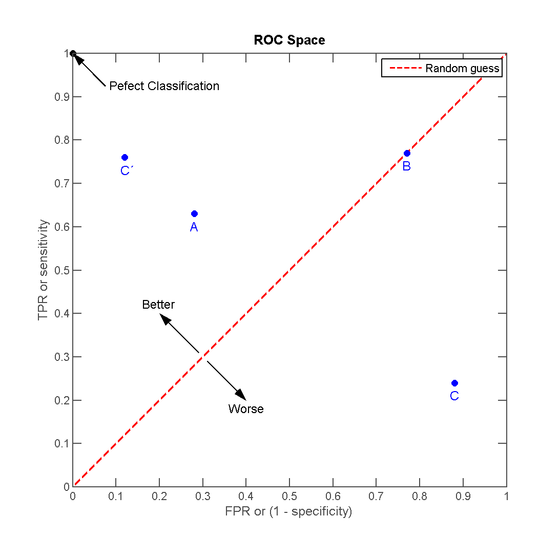
Interpreting the ROC Curve

A curve closer to the diagonal line (random guessing) indicates poor predictive ability.

Interpreting the ROC Curve

The Area Under the Curve (AUC) quantifies the overall model performance, with AUC = 1 being perfect and AUC = 0.5 being no better than chance.

Model Tuning

In e.g. a storm model….
adjusting the model’s decision threshold
- (e.g., how strong a weather signal needs to be before predicting a storm),
- we can move along the ROC curve to balance
  - sensitivity and
  - specificity.

ROC Curve evaluation

Let’s look at our most recent fit:

fit

Generalized Linear Model 

6688 samples
  29 predictor
   2 classes: 'FALSE', 'TRUE' 

No pre-processing
Resampling: Cross-Validated (5 fold) 
Summary of sample sizes: 5351, 5351, 5350, 5349, 5351 
Resampling results:

  Accuracy   Kappa    
  0.8449465  0.6420326

See the curve

prob <- predict(fit, newdata = test, type = "prob")[,2]
myRoc <- roc(test$oregon, prob)
plot(myRoc)

auc(myRoc)

Area under the curve: 0.9175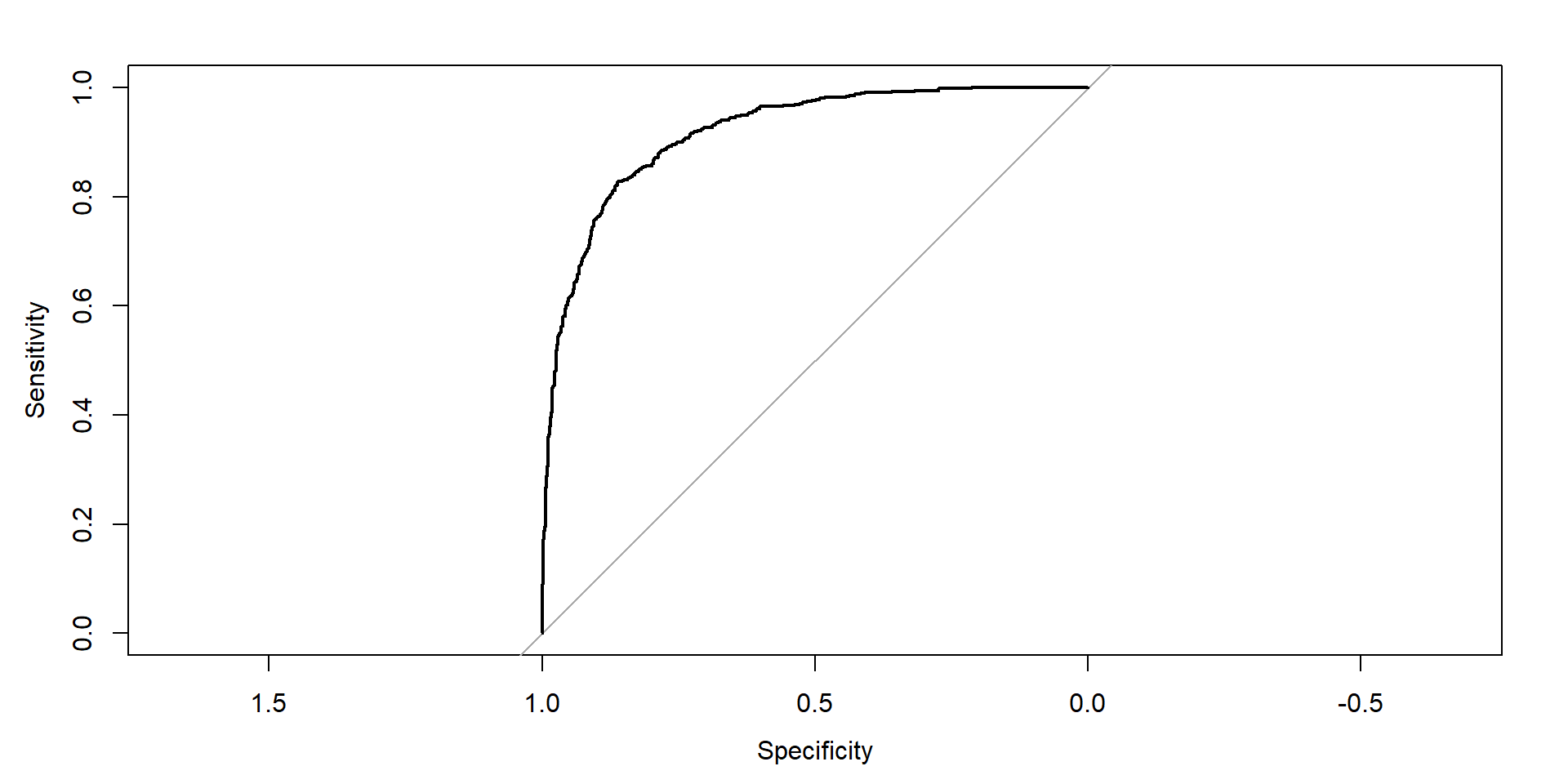

Exercise

Gather into your prediction teams.
Choose a Pinot province other than Oregon or California
Use logistic regression to find the words/terms that increase the odds of choosing that province the most

Vocabulary

Logistic Regression
Odds
Sensitivity
Specificity
ROC
AUC