Dimensionality Reduction

Applied Machine Learning

Jameson > Hendrik > Calvin

Agenda

Review of Mid-term
Next modeling project
Principle component analysis
Topic modeling
Group breakout sessions (if time)

Timing Update

I misnumbered my weeks, so Model 2 is due immediately before the final.
In theory, this means you have more time on it.
Anyways:
- Model 2 by 14 Apr
- Final on 21 Apr

Next modeling project

Due 2 more Mondays (14 Apr)
Use bank data to predict churn
Using only 5 features
Models scored based on AUC
We’ll leave time at the end to get started

Principle component analysis

Principal component analysis (PCA) is a linear dimensionality reduction technique with applications in exploratory data analysis, visualization and data preprocessing.

How?

The data is linearly transformed onto a new coordinate system such that the directions (principal components) capturing the largest variation in the data can be easily identified.

Linear Transform

We use this notion of linear combinations a lot:
- Features with coeffiencients
- Street address
- Course numbers
DATA 505 is a combination of
- a non-numerical (categorical) prefix
- a “hundred level” (5, for MS) and
- a course number (05)

Non-independence

There are many more 100 and 200 level courses than 500
- So we shouldn’t assume that “05” means the same thing after “5” as it does after “1”
  - Many prefixes \(\times\) hundred levels lack an “01” course at all!

Visualize

PCA of a multivariate Gaussian distribution centered at (1,3) with a standard deviation of 3 in roughly the (0.866, 0.5) direction and of 1 in the orthogonal direction. The vectors shown are the eigenvectors of the covariance matrix scaled by the square root of the corresponding eigenvalue, and shifted so their tails are at the mean.

Why?

What are the primary reasons to use PCA?

Dimensionality reduction
Visualization
Noise reduction

Curse of dimensionality

As the dimensionality of the feature space increases,
- the number of configurations can grow exponentially, and thus
- the number of configurations covered by an observation decreases.
Another formulation:
- distances between observations
  - tend to shrink as
  - dimensionality tends to infinity.

src

Idea

Find a linear combination of variables to create principle components
Maintain as much variance as possible.
Principle components are orthogonal (uncorrelated)

Rotation of orthogonal axes

PCA of a multivariate Gaussian distribution centered at (1,3) with a standard deviation of 3 in roughly the (0.866, 0.5) direction and of 1 in the orthogonal direction. The vectors shown are the eigenvectors of the covariance matrix scaled by the square root of the corresponding eigenvalue, and shifted so their tails are at the mean.

Singular value decomposition

Illustration of the singular value decomposition \(U\Sigma V⁎\) of matrix \(M\).
- Top: The action of \(M\), indicated by its effect on the unit disc \(D\) and the two canonical unit vectors \(e_1\) and \(e_2\).
- Left: The action of \(V⁎\), a rotation, on \(D\), \(e_1\) and \(e_2\).
- Bottom: The action of \(\Sigma\), a scaling by the singular values \(\sigma_1\) horizontally and \(\sigma_1\) vertically.
- Right: The action of \(U\), another rotation.

Libraries Setup

Note we are putting id into the wine dataframe!
- Why do we do this?

sh <- suppressPackageStartupMessages
sh(library(tidyverse))
sh(library(tidytext))
sh(library(caret))
sh(library(topicmodels)) # new?
data(stop_words)
sh(library(thematic))
theme_set(theme_dark())
thematic_rmd(bg = "#111", fg = "#eee", accent = "#eee")
wine <- readRDS(gzcon(url("https://cd-public.github.io/D505/dat/variety.rds"))) %>% rowid_to_column("id") 
bank <- readRDS(gzcon(url("https://cd-public.github.io/D505/dat/BankChurners.rds")))

Wine Words

Let’s take some wine words.

winewords <- function(df, cutoff) {
  df %>% 
    unnest_tokens(word, description) %>% anti_join(stop_words) %>%
    filter(!(word %in% c("drink","vineyard","variety","price","points","wine","pinot","chardonnay","gris","noir","riesling","syrah"))) %>% 
    count(id, word) %>%  group_by(word) %>%  mutate(total = sum(n)) %>%  filter(total > cutoff) %>% 
    ungroup() %>% group_by(id) %>% mutate(exists = if_else(n>0,1,0)) %>%  ungroup() %>% 
    pivot_wider(id_cols=id, names_from=word, values_from=exists, values_fill=c(exists=0)) %>% 
    right_join(wine, by="id") %>% drop_na(.) %>%  mutate(log_price = log(price)) %>% 
    select(-id, -price, -description) 
}

Wine Words

Let’s take some wine words.

wino <- winewords(wine, 500)
names(wine)

[1] "id"          "variety"     "price"       "points"      "description"

PCA

prcomp: Principal Components Analysis

Performs a principal components analysis on the given data matrix and returns the results as an object of class prcomp.

PCA the wine

pr_wine <- prcomp(x = select(wino,-variety), scale = T, center = T)
summary(pr_wine)

Importance of components:
                          PC1    PC2    PC3    PC4     PC5     PC6     PC7
Standard deviation     1.3365 1.1225 1.0462 1.0164 0.99785 0.97618 0.95977
Proportion of Variance 0.1786 0.1260 0.1095 0.1033 0.09957 0.09529 0.09212
Cumulative Proportion  0.1786 0.3046 0.4141 0.5174 0.61697 0.71226 0.80438
                           PC8     PC9    PC10
Standard deviation     0.90424 0.84859 0.64691
Proportion of Variance 0.08176 0.07201 0.04185
Cumulative Proportion  0.88614 0.95815 1.00000

Show variance plot

screeplot(pr_wine, type = "lines")

Visualize biplots

biplot(pr_wine)

Visualize biplots

biplot(pr_wine, choices = c(3,4))

Factor loadings

pr_wine$rotation

                  PC1         PC2         PC3          PC4         PC5
flavors   -0.12478797 -0.62231667  0.20452230 -0.318630695  0.13664856
tart      -0.14685952  0.38830520 -0.12183008 -0.280795083 -0.21656122
oak        0.07633205 -0.08679216 -0.68973197  0.099583899 -0.47869174
finish     0.01746794 -0.05286174  0.25007481  0.859753722 -0.07885236
fruit      0.13660189  0.53749981 -0.17969818  0.037421478  0.49610389
tannins    0.11111542  0.27285155  0.47849402 -0.237346398 -0.40926470
cherry     0.37873576  0.14326980  0.24907181 -0.037509702  0.19615664
light     -0.24837285  0.17747080  0.27319253  0.069367578 -0.43069001
points     0.59658742 -0.18887826 -0.05944313 -0.003297401 -0.05847348
log_price  0.60388362 -0.02372061  0.06006730 -0.081066609 -0.24095187
                  PC6         PC7         PC8         PC9        PC10
flavors   -0.04766056  0.05424377  0.11086176 -0.64444967  0.04798526
tart      -0.73492763  0.21914758 -0.15739332 -0.23651461  0.13493716
oak        0.29179417 -0.11495294 -0.19800128 -0.36140534  0.06059095
finish    -0.29384173 -0.08875132 -0.03526432 -0.30446445  0.02840786
fruit      0.18035875 -0.04512780  0.40587621 -0.46049057  0.03563910
tannins    0.13904469 -0.62839693  0.01867847 -0.15124842  0.15158122
cherry     0.24157483  0.30605898 -0.73331841 -0.18300560  0.10408832
light      0.36764429  0.63115133  0.29992812 -0.07632032  0.11215674
points    -0.14532219  0.11863618  0.29334800  0.15866137  0.67455570
log_price -0.14007525  0.15787054  0.20889886 -0.07756363 -0.68725919

Plotly

library(plotly)
biplot_data <- data.frame(pr_wine$x)
biplot_data$variety <- wino$variety

p <- plot_ly(biplot_data, x = ~PC1, y = ~PC2, z = ~PC3, color = ~PC4, type = 'scatter3d', mode = 'markers') %>%
  layout(title = '3D Biplot',
         scene = list(
           xaxis = list(title = 'PC1'),
           yaxis = list(title = 'PC2'),
           zaxis = list(title = 'PC3')
         ))

See it

Add labels

This is a bit objective but you can just look at the biggest positive coefficient.

prc <- bind_cols(select(wino,variety),as.data.frame(pr_wine$x)) %>% 
  select(1:5) %>% 
  rename("points" = PC1) %>% 
  rename("fruit" = PC2) %>% 
  rename("tannin" = PC3) %>% 
  rename("finish" = PC4)
head(prc)

# A tibble: 6 × 5
  variety    points  fruit  tannin finish
  <chr>       <dbl>  <dbl>   <dbl>  <dbl>
1 Pinot_Gris -2.56  -0.453 -0.239  -1.41 
2 Pinot_Noir -1.69   0.547 -2.42   -0.573
3 Pinot_Noir -0.274  0.728  0.0335  1.76 
4 Pinot_Noir -1.52  -0.729  1.52   -1.36 
5 Pinot_Noir -1.68  -1.50   0.195  -0.717
6 Pinot_Noir  1.39   0.213  2.17    0.411

Density by variety (1&2)

prc %>% 
  select(variety, points, fruit) %>% 
  pivot_longer(cols = -variety,names_to = "component",values_to = "loading") %>% 
  ggplot(aes(loading, fill=variety)) +
  geom_density(alpha=0.5) +
  facet_grid(.~component)

Density by variety (3&4)

prc %>% 
  select(variety, tannin, finish) %>% 
  pivot_longer(cols = -variety,names_to = "component",values_to = "loading") %>% 
  ggplot(aes(loading, fill=variety)) +
  geom_density(alpha=0.5) +
  facet_grid(.~component)

Aside

This should be factored.

see_two <- function(df, thing1, thing2) {
  df %>% 
    select(variety, thing1, thing2) %>% 
    pivot_longer(cols = -variety,names_to = "component",values_to = "loading") %>% 
    ggplot(aes(loading, fill=variety)) +
    geom_density(alpha=0.5) +
    facet_grid(.~component)
}

Use it

see_two(prc, "fruit","finish")

More Words

# wino <- winewords(wine, 500)
wino <- winewords(wine, 100)
names(wine)

[1] "id"          "variety"     "price"       "points"      "description"

Why does changing “500” to “100” increase the number of words?

Run PCA

pr_wine <- prcomp(x = select(wino,-variety), scale = T, center = T)
screeplot(pr_wine, type = "lines")

Highest loadings per factor

rownames_to_column(as.data.frame(pr_wine$rotation)) %>% 
  select(1:5) %>% 
  filter(abs(PC1) >= 0.25 | abs(PC2) >= 0.25 | abs(PC3) >= 0.25 | abs(PC4) >= 0.25)

     rowname         PC1        PC2          PC3          PC4
1     months  0.09812814 0.30183350  0.282169826 -0.024209609
2        oak  0.06761861 0.36223058  0.274819423 -0.017899451
3     valley  0.04599743 0.02759857  0.001606928  0.444950984
4       pear -0.25009663 0.13746893 -0.132608010  0.003867835
5     french  0.09425237 0.33440763  0.276955369 -0.034348095
6 willamette  0.04915432 0.02738190 -0.001574066  0.440647855
7     points  0.26481521 0.19037913 -0.326062170  0.030618920
8  log_price  0.36816348 0.02944301 -0.064724155 -0.004236041

Price
French Oak
Also French Oak but not pears or points?
Willamette Valley

Name it

prc <- bind_cols(select(wine,variety),as.data.frame(pr_wine$x)) %>% 
  select(1:5) %>% 
  rename("points"=PC1, "french_oak"=PC2, "french_BROKE"=PC3, "willamette_valley"=PC4)

Graph it

see_two(prc, "points", "willamette_valley")

Graph more

see_two(prc, "french_oak", "french_BROKE")

ML it

fit <- train(variety ~ .,
             data = prc, 
             method = "naive_bayes",
             metric = "Kappa",
             trControl = trainControl(method = "cv"))
confusionMatrix(predict(fit, prc),factor(prc$variety))$overall['Kappa']

    Kappa 
0.6121089

Not bad!

Planned Dinner

Are we close??????

(Long) Exercise

Load the bank data
Run a principal component analysis on all the data except Churn
Choose a number of factors based on a scree plot
name those factors, see whether you can interpret them
Plot them against Churn using a density plot

Hendrik’s solution…

library(fastDummies)
bank <- bank %>%
  mutate(Churn = Churn=="yes") %>%
  dummy_cols(remove_selected_columns = T)
  
pr_bank = prcomp(x = select(bank, -Churn), scale=T, center = T)

Hendrik’s solution…

screeplot(pr_bank, type="lines")

Hendrik’s solution…

rownames_to_column(as.data.frame(pr_bank$rotation)) %>% select(1:5) %>%
  filter(abs(PC1) >= 0.35 | abs(PC2) >= 0.35 | abs(PC3) >= 0.35 | abs(PC4) >= 0.35)

             rowname          PC1         PC2        PC3          PC4
1       Customer_Age -0.010813997  0.07575479 -0.4330194  0.443499234
2     Months_on_book -0.005699747  0.07134628 -0.4278530  0.439072869
3       Credit_Limit  0.413014059 -0.11846478 -0.1156352 -0.003755843
4    Avg_Open_To_Buy  0.416062573 -0.11834914 -0.1350212 -0.033748268
5    Total_Trans_Amt  0.100869534 -0.36992793  0.2898838  0.262444253
6     Total_Trans_Ct  0.044317988 -0.38057169  0.3032594  0.225273171
7           Gender_F -0.355263483 -0.32165703 -0.1903368 -0.067697739
8           Gender_M  0.355263483  0.32165703  0.1903368  0.067697739
9 Card_Category_Blue -0.257857151  0.35138834  0.1591349 -0.022247279

Hendrik’s solution…

prc <- bind_cols(select(bank, Churn), as.data.frame(pr_bank$x)) %>% select(1:5) %>%
  rename("Buy/Credit" = PC1, "Blue/Man" = PC2, "Trans" = PC3, "Age"= PC4)

Hendrik’s solution…

prc %>%
  pivot_longer(cols = -Churn, names_to = "component", values_to = "loading") %>%
  ggplot(aes(loading, fill=Churn)) + geom_density(alpha = 0.5) + facet_grid(.~component)

Topic Modeling

Credit: https://medium.com/data-science/dimensionality-reduction-with-latent-dirichlet-allocation-8d73c586738c

Latent Dirichlet allocation

A common algorithms for topic modeling.
Two principles:
- Every document is a mixture of topics.
- Every topic is a mixture of words.

We imagine that each document may contain words from several topics in particular proportions. For example, in a two-topic model we could say “Document 1 is 90% topic A and 10% topic B, while Document 2 is 30% topic A and 70% topic B.”

Topics

Every topic is a mixture of words. For example, we could imagine a two-topic model of American news, with one topic for “politics” and one for “entertainment.” The most common words in the politics topic might be “President”, “Congress”, and “government”, while the entertainment topic may be made up of words such as “movies”, “television”, and “actor”. Importantly, words can be shared between topics; a word like “budget” might appear in both equally.

Running a model

wine_dtm <- wine %>% 
  unnest_tokens(word, description) %>% anti_join(stop_words) %>%
  filter(!(word %in% c("drink","vineyard","variety","price","points","wine","pinot","chardonnay","gris","noir","riesling","syrah"))) %>% 
  count(id,word) %>% cast_dtm(id, word, n) # DocumentTermMatrix
head(wine_dtm)

<<DocumentTermMatrix (documents: 6, terms: 5836)>>
Non-/sparse entries: 100/34916
Sparsity           : 100%
Maximal term length: 16
Weighting          : term frequency (tf)

Latent Dirichlet

wine_lda <- LDA(wine_dtm, k = 4)#, control = list(seed = 505))
wine_lda

A LDA_VEM topic model with 4 topics.

Introduce two letters.

Lowercase Beta, \(\beta\), per-topic-per-word probabilities
Lowercase Gamma, \(\gamma\), per-document-per-topic probabilities
More
- ctrl+f “beta” and “gamma”
- Use double quotes in the search bar!

Word-topic probabilities

topics <- tidy(wine_lda, matrix = "beta")
head(topics)

# A tibble: 6 × 3
  topic term        beta
  <int> <chr>      <dbl>
1     1 acidity 0.00761 
2     2 acidity 0.00177 
3     3 acidity 0.000637
4     4 acidity 0.00719 
5     1 crisp   0.00357 
6     2 crisp   0.000435

Word-topic probabilities

top_terms <- topics %>%
  group_by(topic) %>% top_n(10, beta) %>% ungroup() %>% arrange(topic, -beta)
top_terms

# A tibble: 40 × 3
   topic term         beta
   <int> <chr>       <dbl>
 1     1 flavors   0.0323 
 2     1 fruit     0.0230 
 3     1 tannins   0.00955
 4     1 tart      0.00932
 5     1 apple     0.00909
 6     1 black     0.00882
 7     1 red       0.00840
 8     1 mix       0.00790
 9     1 acidity   0.00761
10     1 chocolate 0.00736
# ℹ 30 more rows

Word-topic probabilities

plots <- function(df) {
  df %>%
    mutate(term = reorder_within(term, beta, topic)) %>%
    ggplot(aes(term, beta, fill = factor(topic))) +
    geom_col(show.legend = FALSE) +
    facet_wrap(~ topic, scales = "free") +
    coord_flip() +
    scale_x_reordered()
}
plots(top_terms)

Document-topic probabilities

topics <- tidy(wine_lda, matrix = "gamma")
head(topics)

# A tibble: 6 × 3
  document topic gamma
  <chr>    <int> <dbl>
1 1            1 0.254
2 2            1 0.256
3 3            1 0.253
4 4            1 0.249
5 5            1 0.252
6 6            1 0.251

What if we pivot wider?

wider <- function(df) {
  df %>% 
    pivot_wider(id_cols = document,names_from = topic,values_from = gamma, names_prefix = "topic_") %>% 
    mutate(id=as.integer(document)) %>%
    left_join(select(wine, id, variety)) %>% 
    select(-document, -id)
}
topics <- wider(topics)
head(topics)

# A tibble: 6 × 5
  topic_1 topic_2 topic_3 topic_4 variety   
    <dbl>   <dbl>   <dbl>   <dbl> <chr>     
1   0.254   0.247   0.247   0.251 Pinot_Gris
2   0.256   0.252   0.246   0.246 Pinot_Noir
3   0.253   0.249   0.249   0.249 Pinot_Noir
4   0.249   0.249   0.248   0.253 Pinot_Noir
5   0.252   0.252   0.251   0.245 Pinot_Noir
6   0.251   0.258   0.244   0.247 Pinot_Noir

Can we model an outcome?

fit <- train(variety ~ .,
             data = topics, 
             method = "naive_bayes",
             metric = "Kappa",
             trControl = trainControl(method = "cv"),
             maxit = 5)

confusionMatrix(predict(fit, topics),factor(topics$variety))$overall['Kappa']

Kappa 
    0

What if we used more topics?

wine_lda = LDA(wine_dtm, k = 20)
topics <- wider(tidy(wine_lda, matrix = "gamma"))
head(topics)

# A tibble: 6 × 21
  topic_1 topic_2 topic_3 topic_4 topic_5 topic_6 topic_7 topic_8 topic_9
    <dbl>   <dbl>   <dbl>   <dbl>   <dbl>   <dbl>   <dbl>   <dbl>   <dbl>
1  0.0497  0.0501  0.0503  0.0497  0.0502  0.0496  0.0498  0.0499  0.0499
2  0.0502  0.0506  0.0503  0.0495  0.0503  0.0496  0.0498  0.0499  0.0496
3  0.0497  0.0499  0.0501  0.0500  0.0502  0.0497  0.0506  0.0496  0.0497
4  0.0501  0.0497  0.0499  0.0498  0.0504  0.0505  0.0503  0.0504  0.0498
5  0.0502  0.0498  0.0501  0.0503  0.0502  0.0501  0.0504  0.0500  0.0496
6  0.0499  0.0522  0.0502  0.0498  0.0501  0.0498  0.0502  0.0495  0.0495
# ℹ 12 more variables: topic_10 <dbl>, topic_11 <dbl>, topic_12 <dbl>,
#   topic_13 <dbl>, topic_14 <dbl>, topic_15 <dbl>, topic_16 <dbl>,
#   topic_17 <dbl>, topic_18 <dbl>, topic_19 <dbl>, topic_20 <dbl>,
#   variety <chr>

What if we used more topics?

fit <- train(variety ~ .,
             data = topics, 
             method = "naive_bayes",
             metric = "Kappa",
             trControl = trainControl(method = "cv"),
             maxit = 5)

confusionMatrix(predict(fit, topics),factor(topics$variety))$overall['Kappa']

    Kappa 
0.3708219

Associated Press

data("AssociatedPress")
assoc_LDA = LDA(AssociatedPress, k = 2, control = list(seed = 503))

Word-topic probabilities

assoc_topics = tidy(assoc_LDA, matrix="beta")
head(assoc_topics, 20)

# A tibble: 20 × 3
   topic term           beta
   <int> <chr>         <dbl>
 1     1 aaron      3.41e- 5
 2     2 aaron      1.02e- 5
 3     1 abandon    3.94e- 5
 4     2 abandon    2.87e- 5
 5     1 abandoned  4.11e- 5
 6     2 abandoned  1.50e- 4
 7     1 abandoning 1.99e- 5
 8     2 abandoning 6.77e- 6
 9     1 abbott     3.44e- 5
10     2 abbott     7.32e-15
11     1 abboud     3.44e- 5
12     2 abboud     2.72e-45
13     1 abc        2.27e- 4
14     2 abc        6.49e- 5
15     1 abcs       6.80e- 5
16     2 abcs       1.57e- 5
17     1 abctvs     2.55e- 6
18     2 abctvs     3.15e- 5
19     1 abdomen    6.80e- 6
20     2 abdomen    3.65e- 5

Greatest beta differences

assoc_topics %>%
  mutate(topic = paste0("topic", topic)) %>%
  pivot_wider(names_from = topic, values_from = beta) %>%
  head(20)

# A tibble: 20 × 3
   term         topic1   topic2
   <chr>         <dbl>    <dbl>
 1 aaron      3.41e- 5 1.02e- 5
 2 abandon    3.94e- 5 2.87e- 5
 3 abandoned  4.11e- 5 1.50e- 4
 4 abandoning 1.99e- 5 6.77e- 6
 5 abbott     3.44e- 5 7.32e-15
 6 abboud     3.44e- 5 2.72e-45
 7 abc        2.27e- 4 6.49e- 5
 8 abcs       6.80e- 5 1.57e- 5
 9 abctvs     2.55e- 6 3.15e- 5
10 abdomen    6.80e- 6 3.65e- 5
11 abducted   1.78e-10 4.43e- 5
12 abduction  5.02e- 6 3.85e- 5
13 abductors  7.50e-29 2.95e- 5
14 abdul      5.18e- 7 2.89e- 5
15 abide      8.71e- 6 1.96e- 5
16 abilities  3.01e- 5 7.62e- 9
17 ability    1.65e- 4 8.21e- 5
18 ablaze     4.00e-13 6.39e- 5
19 able       3.18e- 4 3.93e- 4
20 abm        6.80e-13 3.44e- 5

Greatest beta differences

beta_wide <- assoc_topics %>%
  mutate(topic = paste0("topic", topic)) %>%
  pivot_wider(names_from = topic, values_from = beta) %>% 
  filter(topic1 > .001 | topic2 > .001) %>%
  mutate(log_ratio = log2(topic2 / topic1))

Greatest beta differences

beta_wide %>%
  head(30)

# A tibble: 30 × 4
   term                 topic1   topic2 log_ratio
   <chr>                 <dbl>    <dbl>     <dbl>
 1 administration 0.00116      0.000796    -0.546
 2 agency         0.000547     0.00118      1.12 
 3 agreement      0.00105      0.000707    -0.564
 4 aid            0.000125     0.00122      3.29 
 5 air            0.000571     0.00160      1.49 
 6 american       0.00204      0.00158     -0.367
 7 area           0.000142     0.00134      3.23 
 8 army           0.0000000371 0.00155     15.4  
 9 arrested       0.0000308    0.00100      5.02 
10 asked          0.000926     0.00108      0.216
# ℹ 20 more rows

Greatest beta differences

ggplot(beta_wide %>% arrange(log_ratio) %>% head(15), aes(x=reorder(term, log_ratio), y=log_ratio)) + 
  geom_bar(stat = "identity") +
  coord_flip()

Greatest beta differences

ggplot(beta_wide %>% arrange(-log_ratio) %>% head(15), aes(x=reorder(term, log_ratio), y=log_ratio)) + 
  geom_bar(stat = "identity") +
  coord_flip()

Credit: https://www.tidytextmining.com/topicmodeling.html

Breakout Sessions

Group modeling project #2! Let’s get started.

Dimensionality Reduction

Agenda

Timing Update

Next modeling project

Principle component analysis

How?

Linear Transform

Non-independence

Visualize

Why?

Curse of dimensionality

Idea

Rotation of orthogonal axes

Singular value decomposition

Libraries Setup

Wine Words

Wine Words

PCA

PCA the wine

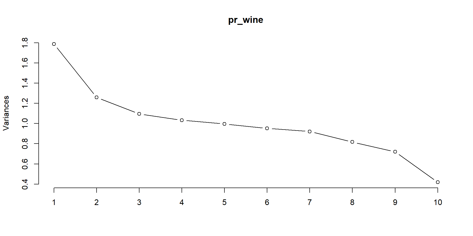
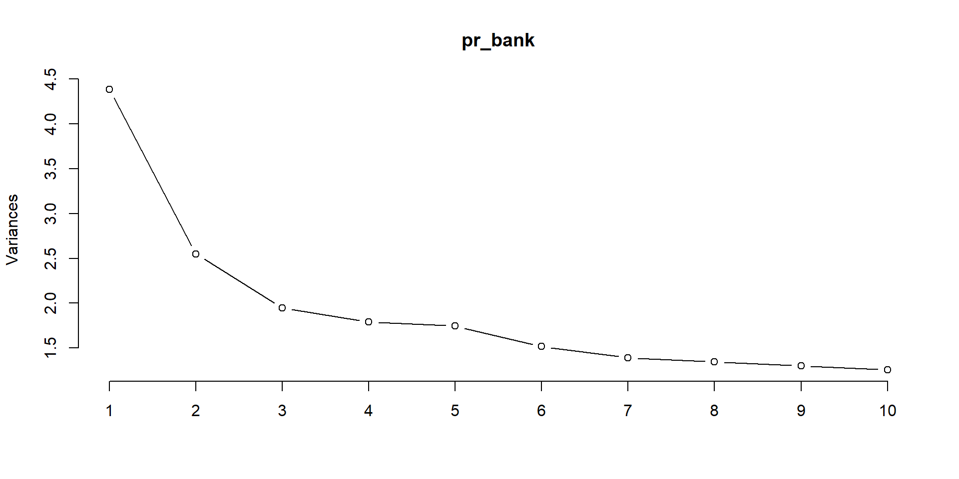
Show variance plot

Visualize biplots

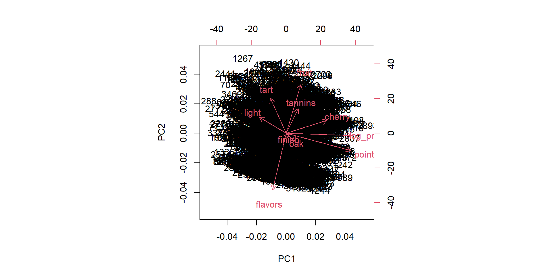
Visualize biplots

Factor loadings

Plotly

See it

Add labels

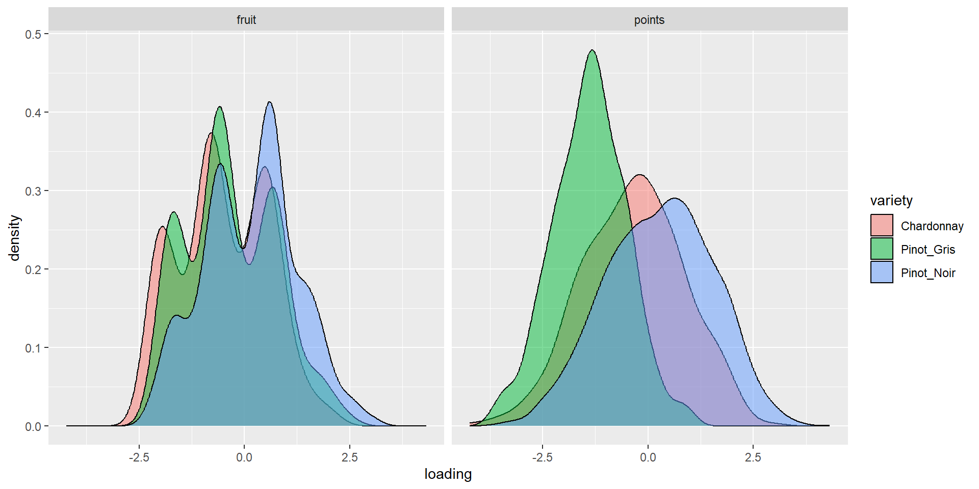
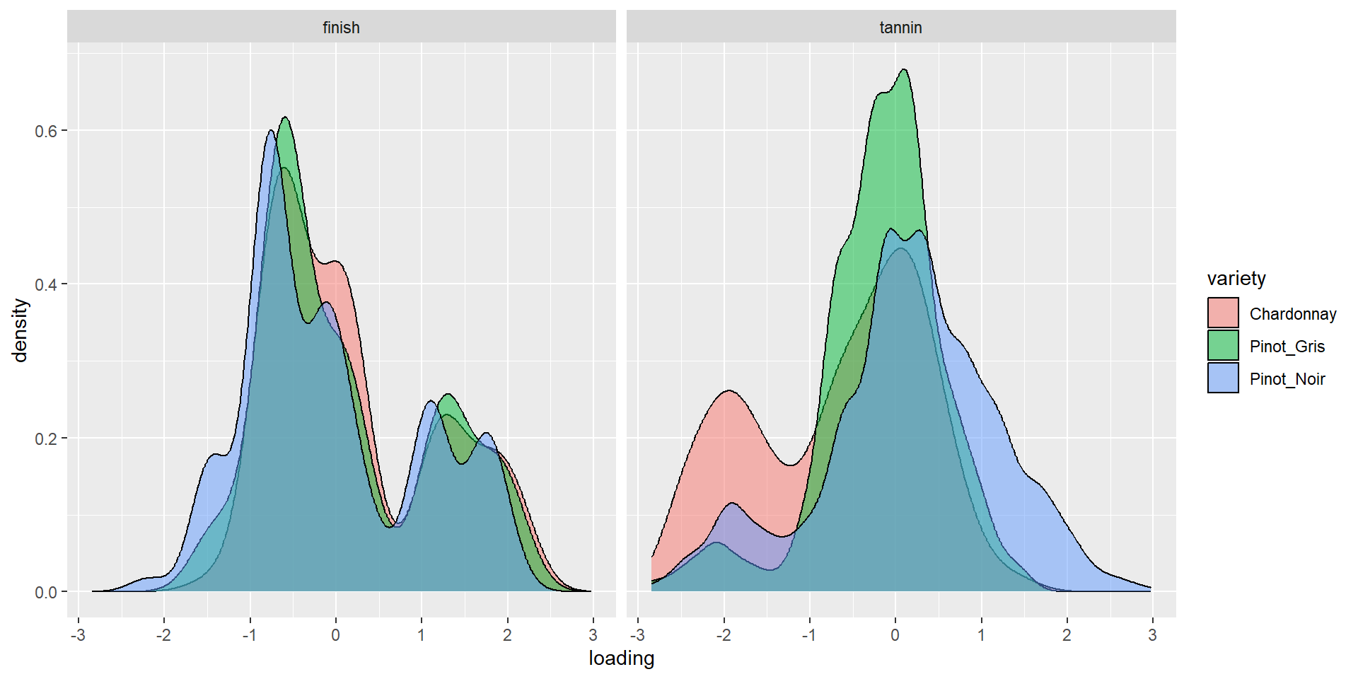
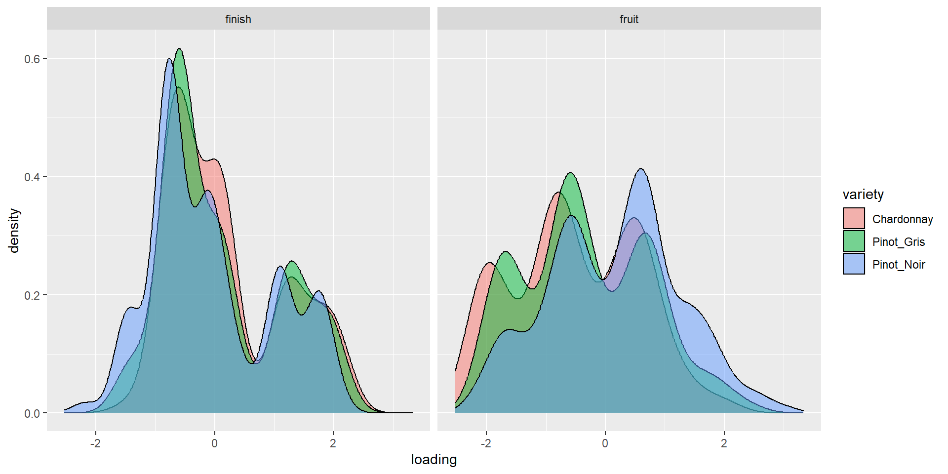
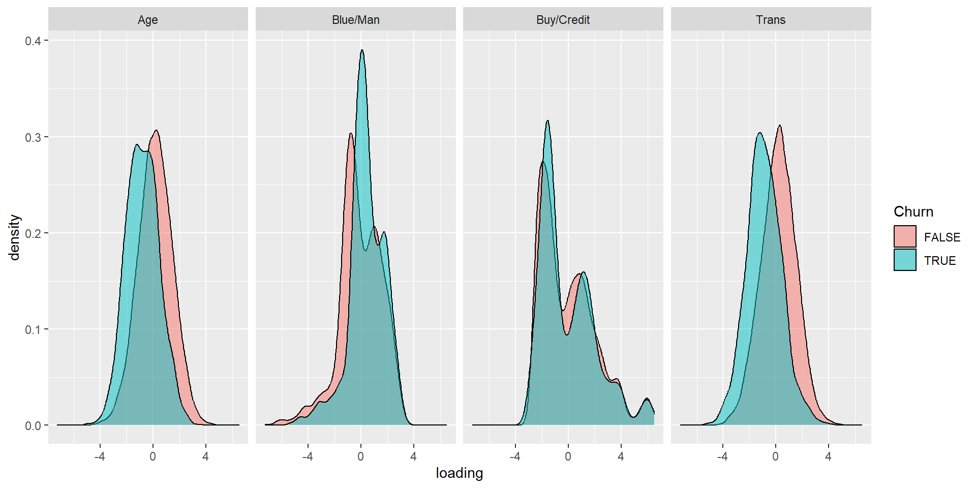
Density by variety (1&2)

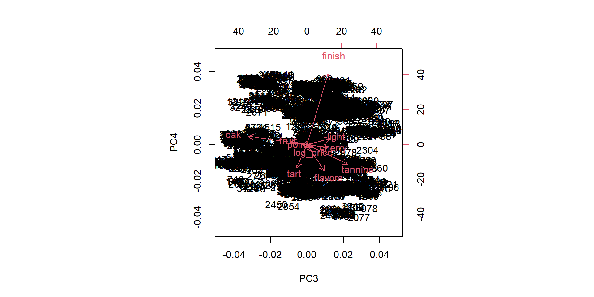
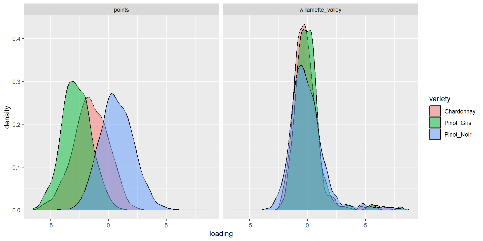
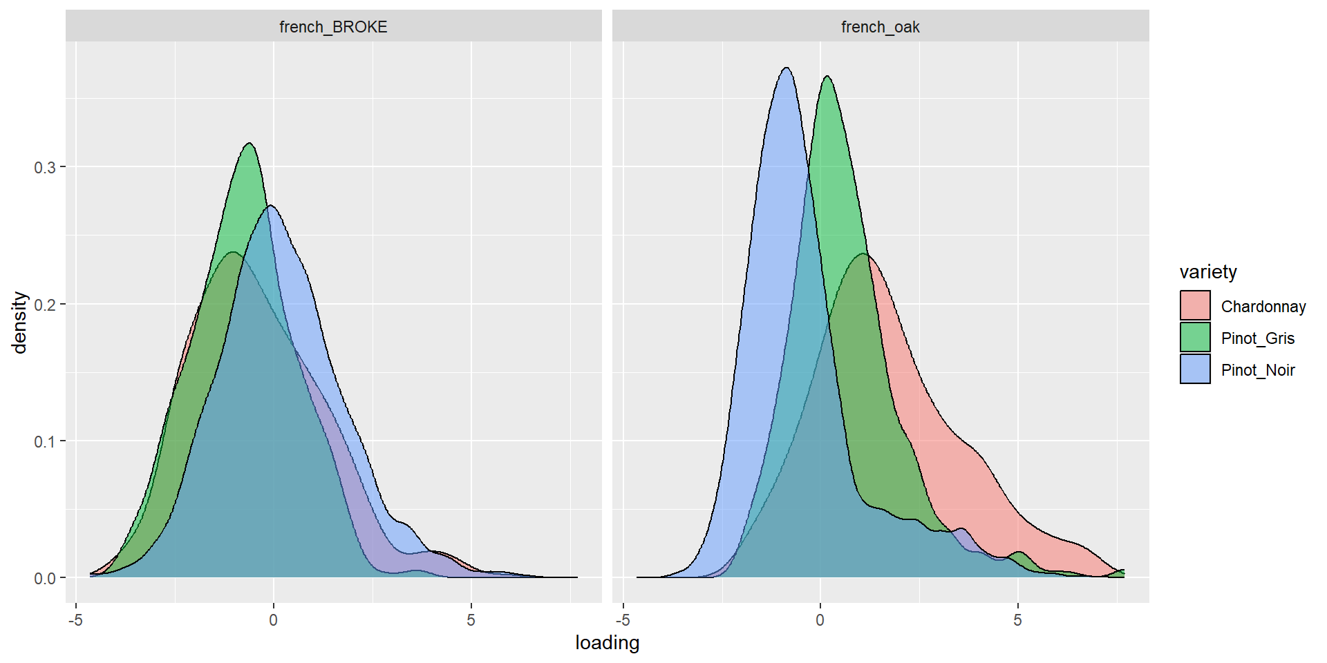
Density by variety (3&4)

Aside

Use it

More Words

Run PCA

Highest loadings per factor

Name it

Graph it

Graph more

ML it

Planned Dinner

(Long) Exercise

Hendrik’s solution…

Hendrik’s solution…

Hendrik’s solution…

Hendrik’s solution…

Hendrik’s solution…

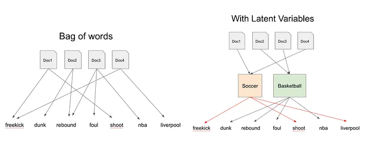
Topic Modeling

Latent Dirichlet allocation

Documents

Topics

Running a model

Latent Dirichlet

Introduce two letters.

Word-topic probabilities

Word-topic probabilities

Word-topic probabilities

Document-topic probabilities

What if we pivot wider?

Can we model an outcome?

What if we used more topics?

What if we used more topics?

Associated Press

Word-topic probabilities

Top words by topic

Greatest beta differences

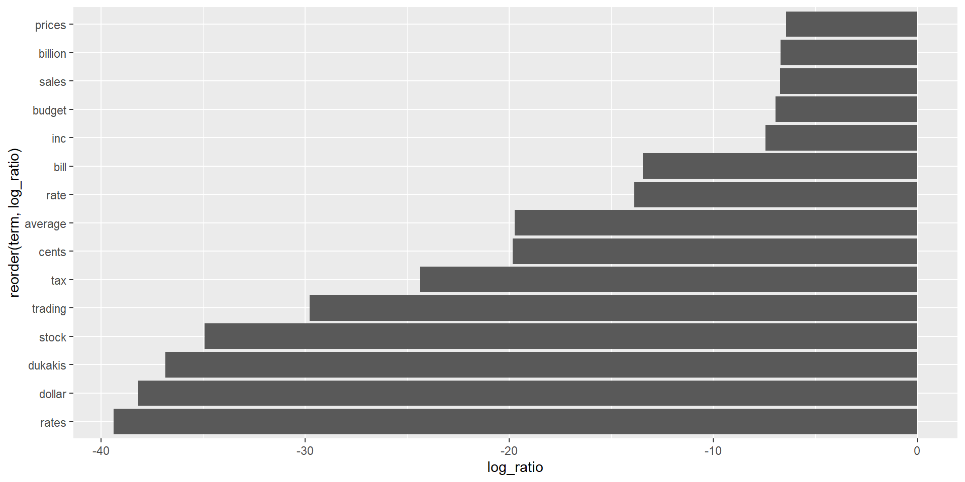
Greatest beta differences

Greatest beta differences

Greatest beta differences

Greatest beta differences

Breakout Sessions