sh <- suppressPackageStartupMessages
sh(library(tidyverse))
sh(library(caret))
sh(library(tidytext))
sh(library(SnowballC))
sh(library(rpart)) # New?
sh(library(randomForest)) # New?
sh(library(doParallel)) # New?
sh(library(gbm)) # New?
data(stop_words)
sh(library(thematic))
theme_set(theme_dark())
thematic_rmd(bg = "#111", fg = "#eee", accent = "#eee")Bagging and Boosting
Applied Machine Learning
Calvin x (Jameson x Hendrik)
Agenda
- Course Announcements
- Weighted models
- Bagged models
- Boosting
- Group work
Midterm 3/17
Brief recap of course so far
- Linear regression (e.g.
lprice ~ .), assumptions of model, interpretation. - \(K\)-NN (e.g.,
province ~ .), multi-class supervised classification. Hyperparameter \(k\). - Naive Bayes (e.g.,
province ~ .), multi-class supervised classification. - Logistic regression (e.g.,
province=="Oregon" ~ .), binary supervised classification. Elastic net. - Feature engineering (logarithms, center/scaling, Box Cox, tidytext, etc.).
- Feature selection (correlation, linear / logistic coefficients, frequent words, frequent words by class, etc.).
Practice
- Practice midterm out.
- You will go over it on 10 Mar.
- It is based on the 5 homeworks.
- It is based on the prior slide.
- Little to no computatational linguistics
- I’m regarding
tidytextas extension, not core, content.
Modality Update
- Reminder for me if we haven’t set modality.
First Model Due 3/10
Publish
- Each group should create:
- An annotated
.*mdfile, and - The .rds/.pickle/.parquet file that it generates, that
- Contains only the features you want in the model.
- Under version control, on GitHub.
Constraints
- I will run:
- The specified \(K\)NN or Naive Bayes model,
- With:
province ~ .(or the whole data frame inscikit) - With repeated 5-fold cross validation
- With the same index for partitioning training and test sets for every group.
- On whatever is turned in before class.
- Bragging rights for highest Kappa
Context
- The “final exam” is that during the last class you will present your model results as though you are speaking to the managers of a large winery.
- It should be presented from a Quarto presentation on GitHub or perhaps e.g. RPubs.
- You must present via the in-room “teaching machine” computer, not your own physical device, to ensure that you are comfortable distributing your findings.
Link up?
- After lecture
Weigted Penalty
Libraries Setup
Dataframe
Wine Words
wine_words <- function(df, j, stem){
  words <- df %>%
    unnest_tokens(word, description) %>%
    anti_join(stop_words) %>%
    filter(!(word %in% c("wine","pinot","vineyard")))

  if(stem){
    words <- words %>% mutate(word = wordStem(word))
  }

  words %>% count(id, word) %>%  group_by(id) %>%  mutate(exists = (n>0)) %>%
    ungroup %>% group_by(word) %>%  mutate(total = sum(n)) %>% filter(total > j) %>%
    pivot_wider(id_cols = id, names_from = word, values_from = exists, values_fill = list(exists=0)) %>%
    right_join(select(df,id,province)) %>% select(-id) %>% mutate(across(-province, ~replace_na(.x, F)))
}
Split It
Quick Training
control = trainControl(method = "cv", number = 5)
fit <- train(province ~ .,
             data = train,
             trControl = control,
             method = "multinom",
             maxit = 5) # speed it up - default 100
# weights: 186 (150 variable)
initial value 9612.789552
final value 4293.654702
stopped after 5 iterations
# weights: 186 (150 variable)
initial value 9612.789552
final value 4298.443311
stopped after 5 iterations
# weights: 186 (150 variable)
initial value 9612.789552
final value 4293.659497
stopped after 5 iterations
# weights: 186 (150 variable)
initial value 9614.581312
final value 4286.131959
stopped after 5 iterations
# weights: 186 (150 variable)
initial value 9614.581312
final value 4290.880467
stopped after 5 iterations
# weights: 186 (150 variable)
initial value 9614.581312
final value 4286.136714
stopped after 5 iterations
# weights: 186 (150 variable)
initial value 9612.789552
final value 4323.482725
stopped after 5 iterations
# weights: 186 (150 variable)
initial value 9612.789552
final value 4328.101450
stopped after 5 iterations
# weights: 186 (150 variable)
initial value 9612.789552
final value 4323.487350
stopped after 5 iterations
# weights: 186 (150 variable)
initial value 9614.581312
final value 4300.974171
stopped after 5 iterations
# weights: 186 (150 variable)
initial value 9614.581312
final value 4305.760565
stopped after 5 iterations
# weights: 186 (150 variable)
initial value 9614.581312
final value 4300.978964
stopped after 5 iterations
# weights: 186 (150 variable)
initial value 9614.581312
final value 4350.524391
stopped after 5 iterations
# weights: 186 (150 variable)
initial value 9614.581312
final value 4355.253533
stopped after 5 iterations
# weights: 186 (150 variable)
initial value 9614.581312
final value 4350.529126
stopped after 5 iterations
# weights: 186 (150 variable)
initial value 12017.330760
final value 5085.731910
stopped after 5 iterationsMatrix
Confusion Matrix and Statistics

                   Reference
Prediction          Burgundy California Casablanca_Valley Marlborough New_York
  Burgundy               181         11                 1           5        2
  California              38        607                 5          18       11
  Casablanca_Valley        0          1                 7           0        0
  Marlborough              0          0                 0           1        0
  New_York                 0          0                 0           0        0
  Oregon                  19        172                13          21       13
                   Reference
Prediction          Oregon
  Burgundy              28
  California            83
  Casablanca_Valley      1
  Marlborough            0
  New_York               0
  Oregon               435

Overall Statistics

               Accuracy : 0.7358
                 95% CI : (0.714, 0.7568)
    No Information Rate : 0.4728
    P-Value [Acc > NIR] : < 2.2e-16

                  Kappa : 0.5831

 Mcnemar's Test P-Value : NA

Statistics by Class:

                     Class: Burgundy Class: California Class: Casablanca_Valley
Sensitivity                   0.7605            0.7674                 0.269231
Specificity                   0.9672            0.8243                 0.998786
Pos Pred Value                0.7939            0.7966                 0.777778
Neg Pred Value                0.9606            0.7980                 0.988582
Prevalence                    0.1423            0.4728                 0.015541
Detection Rate                0.1082            0.3628                 0.004184
Detection Prevalence          0.1363            0.4555                 0.005380
Balanced Accuracy             0.8639            0.7958                 0.634008
                     Class: Marlborough Class: New_York Class: Oregon
Sensitivity                   0.0222222         0.00000        0.7952
Specificity                   1.0000000         1.00000        0.7886
Pos Pred Value                1.0000000             NaN        0.6464
Neg Pred Value                0.9736842         0.98446        0.8880
Prevalence                    0.0268978         0.01554        0.3270
Detection Rate                0.0005977         0.00000        0.2600
Detection Prevalence          0.0005977         0.00000        0.4023
Balanced Accuracy             0.5111111         0.50000        0.7919
Create some weights
Add weight to model
- Look closely:
- Train over
traindataframe - Provide weights from
weight_traindata frame - That way it won’t train on weights!
- Train over
fit <- train(province ~ .,
             data = train,
             trControl = control,
             method = "multinom",
             maxit = 5,
             weights = weight_train$weights)
# weights: 186 (150 variable)
initial value 105991.531402
final value 48035.564209
stopped after 5 iterations
# weights: 186 (150 variable)
initial value 105991.531402
final value 48040.946734
stopped after 5 iterations
# weights: 186 (150 variable)
initial value 105991.531402
final value 48035.569592
stopped after 5 iterations
# weights: 186 (150 variable)
initial value 105991.531402
final value 46545.313878
stopped after 5 iterations
# weights: 186 (150 variable)
initial value 105991.531402
final value 46550.591504
stopped after 5 iterations
# weights: 186 (150 variable)
initial value 105991.531402
final value 46545.319156
stopped after 5 iterations
# weights: 186 (150 variable)
initial value 105989.739643
final value 48068.956223
stopped after 5 iterations
# weights: 186 (150 variable)
initial value 105989.739643
final value 48074.276422
stopped after 5 iterations
# weights: 186 (150 variable)
initial value 105989.739643
final value 48068.961544
stopped after 5 iterations
# weights: 186 (150 variable)
initial value 105989.739643
final value 45944.777964
stopped after 5 iterations
# weights: 186 (150 variable)
initial value 105989.739643
final value 45950.193395
stopped after 5 iterations
# weights: 186 (150 variable)
initial value 105989.739643
final value 45944.783380
stopped after 5 iterations
# weights: 186 (150 variable)
initial value 106025.574832
final value 48603.782942
stopped after 5 iterations
# weights: 186 (150 variable)
initial value 106025.574832
final value 48609.093526
stopped after 5 iterations
# weights: 186 (150 variable)
initial value 106025.574832
final value 48603.788253
stopped after 5 iterations
# weights: 186 (150 variable)
initial value 132497.029230
final value 51901.008448
stopped after 5 iterationsMatrix
Confusion Matrix and Statistics

                   Reference
Prediction          Burgundy California Casablanca_Valley Marlborough New_York
  Burgundy               221         98                 1           6        6
  California               0        211                 0           1        2
  Casablanca_Valley        2         20                18           0        5
  Marlborough              2        135                 0          23        5
  New_York                 0         16                 0           1        5
  Oregon                  13        311                 7          14        3
                   Reference
Prediction          Oregon
  Burgundy              60
  California             3
  Casablanca_Valley      3
  Marlborough           21
  New_York               2
  Oregon               458

Overall Statistics

               Accuracy : 0.5595
                 95% CI : (0.5353, 0.5834)
    No Information Rate : 0.4728
    P-Value [Acc > NIR] : 7.657e-13

                  Kappa : 0.408

 Mcnemar's Test P-Value : NA

Statistics by Class:

                     Class: Burgundy Class: California Class: Casablanca_Valley
Sensitivity                   0.9286            0.2668                  0.69231
Specificity                   0.8808            0.9932                  0.98179
Pos Pred Value                0.5638            0.9724                  0.37500
Neg Pred Value                0.9867            0.6016                  0.99508
Prevalence                    0.1423            0.4728                  0.01554
Detection Rate                0.1321            0.1261                  0.01076
Detection Prevalence          0.2343            0.1297                  0.02869
Balanced Accuracy             0.9047            0.6300                  0.83705
                     Class: Marlborough Class: New_York Class: Oregon
Sensitivity                     0.51111        0.192308        0.8373
Specificity                     0.89988        0.988464        0.6909
Pos Pred Value                  0.12366        0.208333        0.5682
Neg Pred Value                  0.98521        0.987265        0.8973
Prevalence                      0.02690        0.015541        0.3270
Detection Rate                  0.01375        0.002989        0.2738
Detection Prevalence            0.11118        0.014345        0.4818
Balanced Accuracy               0.70549        0.590386        0.7641
Weighted Models
- Where do these weights come from?
Progressive overload
fit <- train(province ~ .,
             data = train,
             trControl = control,
             method = "multinom",
             maxit = 5,
             weights = weight_train$weights)
# weights: 186 (150 variable)
initial value 29052.125562
final value 14594.434569
stopped after 5 iterations
# weights: 186 (150 variable)
initial value 29052.125562
final value 14600.444684
stopped after 5 iterations
# weights: 186 (150 variable)
initial value 29052.125562
final value 14594.440582
stopped after 5 iterations
# weights: 186 (150 variable)
initial value 29085.273112
final value 15333.346364
stopped after 5 iterations
# weights: 186 (150 variable)
initial value 29085.273112
final value 15339.437606
stopped after 5 iterations
# weights: 186 (150 variable)
initial value 29085.273112
final value 15333.352458
stopped after 5 iterations
# weights: 186 (150 variable)
initial value 29053.917321
final value 15053.131982
stopped after 5 iterations
# weights: 186 (150 variable)
initial value 29053.917321
final value 15059.407508
stopped after 5 iterations
# weights: 186 (150 variable)
initial value 29053.917321
final value 15053.138261
stopped after 5 iterations
# weights: 186 (150 variable)
initial value 29052.125562
final value 15366.545546
stopped after 5 iterations
# weights: 186 (150 variable)
initial value 29052.125562
final value 15372.704878
stopped after 5 iterations
# weights: 186 (150 variable)
initial value 29052.125562
final value 15366.551708
stopped after 5 iterations
# weights: 186 (150 variable)
initial value 29053.917321
final value 14871.524669
stopped after 5 iterations
# weights: 186 (150 variable)
initial value 29053.917321
final value 14877.593414
stopped after 5 iterations
# weights: 186 (150 variable)
initial value 29053.917321
final value 14871.530741
stopped after 5 iterations
# weights: 186 (150 variable)
initial value 36324.339720
final value 19122.264208
stopped after 5 iterationsMatrix
Confusion Matrix and Statistics

                   Reference
Prediction          Burgundy California Casablanca_Valley Marlborough New_York
  Burgundy               215         82                 1           8        4
  California               0        378                 0           2        0
  Casablanca_Valley        2         48                22           1        7
  Marlborough              0         13                 0          12        0
  New_York                 6         94                 0           7       12
  Oregon                  15        176                 3          15        3
                   Reference
Prediction          Oregon
  Burgundy              70
  California            15
  Casablanca_Valley      9
  Marlborough            4
  New_York              16
  Oregon               433

Overall Statistics

               Accuracy : 0.6408
                 95% CI : (0.6172, 0.6638)
    No Information Rate : 0.4728
    P-Value [Acc > NIR] : < 2.2e-16

                  Kappa : 0.5062

 Mcnemar's Test P-Value : < 2.2e-16

Statistics by Class:

                     Class: Burgundy Class: California Class: Casablanca_Valley
Sensitivity                   0.9034            0.4779                  0.84615
Specificity                   0.8850            0.9807                  0.95932
Pos Pred Value                0.5658            0.9570                  0.24719
Neg Pred Value                0.9822            0.6768                  0.99747
Prevalence                    0.1423            0.4728                  0.01554
Detection Rate                0.1285            0.2259                  0.01315
Detection Prevalence          0.2271            0.2361                  0.05320
Balanced Accuracy             0.8942            0.7293                  0.90274
                     Class: Marlborough Class: New_York Class: Oregon
Sensitivity                    0.266667        0.461538        0.7916
Specificity                    0.989558        0.925319        0.8117
Pos Pred Value                 0.413793        0.088889        0.6713
Neg Pred Value                 0.979927        0.990897        0.8891
Prevalence                     0.026898        0.015541        0.3270
Detection Rate                 0.007173        0.007173        0.2588
Detection Prevalence           0.017334        0.080693        0.3855
Balanced Accuracy              0.628112        0.693429        0.8017
Weight generation
- Check wines per province.
Exercise
- Write a function to:
- Find weights, given
- A dataframe, and
- A column name.
Regularization

Penalty
- Regularization is often also called ‘penalization’ because it adds a penalizing term to the loss function.
\[ \min_{f}\sum_{i=1}^{n}V(f(x_{i}),y_{i})+\lambda R(f) \]
- De facto application of Occam’s Razor.
- Assume simple is good.
- Therefore punish coefficients (which complicate things)
Penalties
- The amount of the penalty is fine-tuned using a constant lambda \(\lambda\).
- When \(\lambda = 0\), no penalty is enforced.
- The best lambda can be found by finding a value that minimizes prediction error after cross validating the model with different values.
Lasso Regression
- Given \(p\) features and \(N\) observations.
- \(\beta\)’s are coefficients.
- The \(\lambda\) term is evaluated via absolute value \(|\beta_j|\)
\[ \sum_{i=1}^{n} \left( y_i - \beta_0 - \sum_{j=1}^{p} \beta_j x_{ij} \right) ^ 2 + \lambda \sum_{j=1}^{p} |\beta_j| \]
LASSO
- Least Absolute Shrinkage and Selection Operator.
- Shrinks the regression coefficients toward zero.
- Penalizing the regression model with a penalty term called L1-norm
- The sum of the absolute coefficients.
- I learned about L1 in a class called “Real Analysis”
- Its the streetmap distance (roads and avenues)
Lasso Regression
- Zeroes out some coefficients
- With a minor contribution to the model, can’t “resist” the penalty.
- Lasso can be also seen as an alternative to the subset selection methods.
- A form of variable selection.
glmnet
- “Lasso and Elastic-Net Regularized Generalized Linear Models”
- Elastic-Net on forthcoming slides!
- Use via
- It accepts an
alphavalue.- Set to
1for LASSO - Set to non-one on latter slides!
- Set to
LASSO
tuneGridis I think, clunky, but we only use it here as a demo.
Inspect \(\lambda\)
Confusion Matrix
Confusion Matrix and Statistics

                   Reference
Prediction          Burgundy California Casablanca_Valley Marlborough New_York
  Burgundy               197          6                 0           3        1
  California              15        690                 5          17       14
  Casablanca_Valley        0          2                17           0        1
  Marlborough              0          4                 0           9        0
  New_York                 0          2                 0           0        4
  Oregon                  26         87                 4          16        6
                   Reference
Prediction          Oregon
  Burgundy              24
  California            88
  Casablanca_Valley      2
  Marlborough            2
  New_York               0
  Oregon               431

Overall Statistics

               Accuracy : 0.8057
                 95% CI : (0.786, 0.8244)
    No Information Rate : 0.4728
    P-Value [Acc > NIR] : < 2.2e-16

                  Kappa : 0.6937

 Mcnemar's Test P-Value : NA

Statistics by Class:

                     Class: Burgundy Class: California Class: Casablanca_Valley
Sensitivity                   0.8277            0.8723                  0.65385
Specificity                   0.9763            0.8424                  0.99696
Pos Pred Value                0.8528            0.8323                  0.77273
Neg Pred Value                0.9716            0.8803                  0.99455
Prevalence                    0.1423            0.4728                  0.01554
Detection Rate                0.1178            0.4124                  0.01016
Detection Prevalence          0.1381            0.4955                  0.01315
Balanced Accuracy             0.9020            0.8574                  0.82541
                     Class: Marlborough Class: New_York Class: Oregon
Sensitivity                    0.200000        0.153846        0.7879
Specificity                    0.996314        0.998786        0.8766
Pos Pred Value                 0.600000        0.666667        0.7561
Neg Pred Value                 0.978287        0.986803        0.8948
Prevalence                     0.026898        0.015541        0.3270
Detection Rate                 0.005380        0.002391        0.2576
Detection Prevalence           0.008966        0.003586        0.3407
Balanced Accuracy              0.598157        0.576316        0.8322
Ridge Regression
- Given \(p\) features and \(N\) observations.
- \(\beta\)’s are coefficients.
- The \(\lambda\) term is evaluated via square \(\beta_j^2\)
\[ \sum_{i=1}^{n} \left( y_i - \beta_0 - \sum_{j=1}^{p} \beta_j x_{ij} \right) ^ 2 + \lambda \sum_{j=1}^{p} \beta_j^2 \]
Ridge
- Also Tikhonov regularization, named for Andrey Tikhonov
- Shrinks the regression coefficients toward zero.
- Penalizing the regression model with a penalty term called L2-norm
- The sum of the sqared coefficients.
- I also learned about L2 in “Real Analysis”
- Its the as-birds-fly distance (point-to-point)
Ridge
- Set
alpha(that is, \(\alpha\)) to 0.
Inspect \(\lambda\)
- Much higher than Lasso (0.012 vs 0.001)
Confusion Matrix
Confusion Matrix and Statistics

                   Reference
Prediction          Burgundy California Casablanca_Valley Marlborough New_York
  Burgundy               192          3                 0           3        1
  California              16        698                11          21       17
  Casablanca_Valley        0          0                 8           0        0
  Marlborough              0          4                 0           3        0
  New_York                 0          1                 0           0        2
  Oregon                  30         85                 7          18        6
                   Reference
Prediction          Oregon
  Burgundy              19
  California            90
  Casablanca_Valley      1
  Marlborough            0
  New_York               0
  Oregon               437

Overall Statistics

               Accuracy : 0.801
                 95% CI : (0.781, 0.8198)
    No Information Rate : 0.4728
    P-Value [Acc > NIR] : < 2.2e-16

                  Kappa : 0.6822

 Mcnemar's Test P-Value : NA

Statistics by Class:

                     Class: Burgundy Class: California Class: Casablanca_Valley
Sensitivity                   0.8067            0.8824                 0.307692
Specificity                   0.9819            0.8243                 0.999393
Pos Pred Value                0.8807            0.8183                 0.888889
Neg Pred Value                0.9684            0.8866                 0.989183
Prevalence                    0.1423            0.4728                 0.015541
Detection Rate                0.1148            0.4172                 0.004782
Detection Prevalence          0.1303            0.5099                 0.005380
Balanced Accuracy             0.8943            0.8533                 0.653543
                     Class: Marlborough Class: New_York Class: Oregon
Sensitivity                    0.066667        0.076923        0.7989
Specificity                    0.997543        0.999393        0.8703
Pos Pred Value                 0.428571        0.666667        0.7496
Neg Pred Value                 0.974790        0.985629        0.8991
Prevalence                     0.026898        0.015541        0.3270
Detection Rate                 0.001793        0.001195        0.2612
Detection Prevalence           0.004184        0.001793        0.3485
Balanced Accuracy              0.532105        0.538158        0.8346
Elastic Net
- Given \(p\) features and \(N\) observations.
- \(\beta\)’s are coefficients.
- Add both together and weight them comparatively via parameter \(\alpha\)
- Lower case alpha.
\[ \sum_{i=1}^{n} \left( y_i - \beta_0 - \sum_{j=1}^{p} \beta_j x_{ij} \right) ^ 2 + \alpha\lambda \sum_{j=1}^{p} |\beta_j|+(1-\alpha)\lambda \sum_{j=1}^{p} \beta_j^2 \]
Deciding
- I only ever hear of LASSO or elastic net, which combines Lasso and Ridge:
- Lasso better in a situation where some of the predictors have large coefficients, and the remaining predictors have very small coefficients.
- Ridge regression better when many predictors with coefficients of roughly equal size.
- Not too costly to just try them or tune along \(\alpha\)
Elastic Net
- This is the fun one.
- Just don’t say anything and you get elastic net.
Inspect \(\lambda\) and \(\alpha\)
- Much higher than Lasso (0.012 vs 0.001)
Confusion Matrix
- In this case, doesn’t seem better than Lasso by much at all!
- But - it’s automatic.
- Let the computer think hard so you can spend time thinking about, say, features.
Confusion Matrix and Statistics

                   Reference
Prediction          Burgundy California Casablanca_Valley Marlborough New_York
  Burgundy               194          5                 0           3        1
  California              15        692                 6          17       15
  Casablanca_Valley        0          2                15           0        1
  Marlborough              0          4                 0           9        0
  New_York                 0          3                 0           0        3
  Oregon                  29         85                 5          16        6
                   Reference
Prediction          Oregon
  Burgundy              23
  California            90
  Casablanca_Valley      1
  Marlborough            1
  New_York               0
  Oregon               432

Overall Statistics

               Accuracy : 0.8039
                 95% CI : (0.7841, 0.8227)
    No Information Rate : 0.4728
    P-Value [Acc > NIR] : < 2.2e-16

                  Kappa : 0.69

 Mcnemar's Test P-Value : NA

Statistics by Class:

                     Class: Burgundy Class: California Class: Casablanca_Valley
Sensitivity                   0.8151            0.8748                 0.576923
Specificity                   0.9777            0.8379                 0.997571
Pos Pred Value                0.8584            0.8287                 0.789474
Neg Pred Value                0.9696            0.8819                 0.993349
Prevalence                    0.1423            0.4728                 0.015541
Detection Rate                0.1160            0.4136                 0.008966
Detection Prevalence          0.1351            0.4991                 0.011357
Balanced Accuracy             0.8964            0.8564                 0.787247
                     Class: Marlborough Class: New_York Class: Oregon
Sensitivity                    0.200000        0.115385        0.7898
Specificity                    0.996929        0.998179        0.8748
Pos Pred Value                 0.642857        0.500000        0.7539
Neg Pred Value                 0.978300        0.986203        0.8955
Prevalence                     0.026898        0.015541        0.3270
Detection Rate                 0.005380        0.001793        0.2582
Detection Prevalence           0.008368        0.003586        0.3425
Balanced Accuracy              0.598464        0.556782        0.8323
Bagging, Boosting and Custom Ensembles
Understanding the Bias-Variance Tradeoff by Scott Fortman-Roe
| Low Variance | High Variance | |
| Low Bias | ||
| High Bias |
Goals
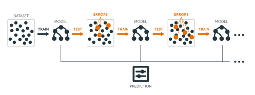
The goal is to decrease the variance (bagging) or bias (boosting) in our models.
- Step 1: producing a distribution of simple ML models on subsets of the original data.
- Step 2: combine the distribution into one “aggregated” model.
Framework
Note: Subtle difference between Bagging/Boosting and resampling.
- Re-sampling –> average coefficients from different subsamples to create one model
- Bagging/Boosting –> average the predictions from different models
Bagging (subsets of data)
- “Bootstrap aggregating”
- Builds multiple models with bootstrap samples (combinations with repetitions) using a single algorithm.
- The models’ predictions are combined with voting (for classification) or averaging (for numeric prediction).
- Voting means the bagging model’s prediction is based on the majority of learners’ prediction for a class.
Bagging

Treebag
- Treebag, or, generate trees and combine trees, taking different weights.
fit <- train(province ~ .,
             data = train,
             trControl = control,
             method = "treebag",
             maxit = 5) # speed it up - default 100
fit
Bagged CART
6707 samples
29 predictor
6 classes: 'Burgundy', 'California', 'Casablanca_Valley', 'Marlborough', 'New_York', 'Oregon'
No pre-processing
Resampling: Cross-Validated (5 fold)
Summary of sample sizes: 5365, 5365, 5367, 5365, 5366
Resampling results:
Accuracy Kappa
0.7835129 0.6621207Confusion Matrix
Confusion Matrix and Statistics

                   Reference
Prediction          Burgundy California Casablanca_Valley Marlborough New_York
  Burgundy               182         11                 0           2        1
  California              16        674                 7          13       14
  Casablanca_Valley        1          3                15           0        2
  Marlborough              1          7                 0          19        2
  New_York                 1          4                 0           0        4
  Oregon                  37         92                 4          11        3
                   Reference
Prediction          Oregon
  Burgundy              28
  California            93
  Casablanca_Valley      2
  Marlborough            3
  New_York               1
  Oregon               420

Overall Statistics

               Accuracy : 0.7854
                 95% CI : (0.765, 0.8049)
    No Information Rate : 0.4728
    P-Value [Acc > NIR] : < 2.2e-16

                  Kappa : 0.6639

 Mcnemar's Test P-Value : NA

Statistics by Class:

                     Class: Burgundy Class: California Class: Casablanca_Valley
Sensitivity                   0.7647            0.8521                 0.576923
Specificity                   0.9707            0.8379                 0.995143
Pos Pred Value                0.8125            0.8250                 0.652174
Neg Pred Value                0.9614            0.8633                 0.993333
Prevalence                    0.1423            0.4728                 0.015541
Detection Rate                0.1088            0.4029                 0.008966
Detection Prevalence          0.1339            0.4883                 0.013748
Balanced Accuracy             0.8677            0.8450                 0.786033
                     Class: Marlborough Class: New_York Class: Oregon
Sensitivity                     0.42222        0.153846        0.7678
Specificity                     0.99201        0.996357        0.8694
Pos Pred Value                  0.59375        0.400000        0.7407
Neg Pred Value                  0.98416        0.986771        0.8852
Prevalence                      0.02690        0.015541        0.3270
Detection Rate                  0.01136        0.002391        0.2510
Detection Prevalence            0.01913        0.005977        0.3389
Balanced Accuracy               0.70712        0.575102        0.8186
Boosting
A horse-racing gambler, hoping to maximize his winnings, decides to create a computer program that will accurately predict the winner of a horse race based on the usual information (number of races recently won by each horse, betting odds for each horse, etc.). To create such a program, he asks a highly successful expert gambler to explain his betting strategy. Not surprisingly, the expert is unable to articulate a grand set of rules for selecting a horse. On the other hand, when presented with the data for a specific set of races, the expert has no trouble coming up with a “rule of thumb” for that set of races (such as, “Bet on the horse that has recently won the most races” or “Bet on the horse with the most favored odds”). Although such a rule of thumb, by itself, is obviously very rough and inaccurate, it is not unreasonable to expect it to provide predictions that are at least a little bit better than random guessing. Furthermore, by repeatedly asking the expert’s opinion on different collections of races, the gambler is able to extract many rules of thumb.
Boosting
In order to use these rules of thumb to maximum advantage, there are two problems faced by the gambler:
First, how should he choose the collections of races presented to the expert so as to extract rules of thumb from the expert that will be the most useful?
Second, once he has collected many rules of thumb, how can they be combined into a single, highly accurate prediction rule?
Boosting refers to a general and provably effective method of producing a very accurate prediction rule by combining rough and moderately inaccurate rules of thumb in a manner similar to that suggested above
Boosting
Boosting
GBM
- Generalized Boost Models are Caret compatible
- XGBoost is more common but requires learning XGB
- It uses different performance acceleration.
- This thing is slow so we modify the defaults:
Boost City
Iter TrainDeviance ValidDeviance StepSize Improve
1 1.7918 nan 0.0100 0.0337
2 1.7734 nan 0.0100 0.0323
3 1.7555 nan 0.0100 0.0310
4 1.7384 nan 0.0100 0.0305
5 1.7219 nan 0.0100 0.0292
6 1.7059 nan 0.0100 0.0282
7 1.6905 nan 0.0100 0.0277
8 1.6753 nan 0.0100 0.0269
9 1.6607 nan 0.0100 0.0263
10 1.6464 nan 0.0100 0.0257
Iter TrainDeviance ValidDeviance StepSize Improve
1 1.7918 nan 0.0100 0.0447
2 1.7665 nan 0.0100 0.0429
3 1.7424 nan 0.0100 0.0408
4 1.7192 nan 0.0100 0.0395
5 1.6968 nan 0.0100 0.0384
6 1.6752 nan 0.0100 0.0366
7 1.6545 nan 0.0100 0.0351
8 1.6348 nan 0.0100 0.0340
9 1.6153 nan 0.0100 0.0331
10 1.5965 nan 0.0100 0.0321
Iter TrainDeviance ValidDeviance StepSize Improve
1 1.7918 nan 0.1000 0.3040
2 1.6166 nan 0.1000 0.2231
3 1.4855 nan 0.1000 0.1611
4 1.3902 nan 0.1000 0.1356
5 1.3107 nan 0.1000 0.1072
6 1.2487 nan 0.1000 0.0885
7 1.1952 nan 0.1000 0.0753
8 1.1495 nan 0.1000 0.0631
9 1.1116 nan 0.1000 0.0514
10 1.0806 nan 0.1000 0.0519
Iter TrainDeviance ValidDeviance StepSize Improve
1 1.7918 nan 0.1000 0.3868
2 1.5589 nan 0.1000 0.2768
3 1.3945 nan 0.1000 0.2037
4 1.2728 nan 0.1000 0.1553
5 1.1791 nan 0.1000 0.1307
6 1.1005 nan 0.1000 0.1040
7 1.0380 nan 0.1000 0.0885
8 0.9844 nan 0.1000 0.0739
9 0.9390 nan 0.1000 0.0633
10 0.8998 nan 0.1000 0.0543
Iter TrainDeviance ValidDeviance StepSize Improve
1 1.7918 nan 0.0100 0.0344
2 1.7731 nan 0.0100 0.0331
3 1.7549 nan 0.0100 0.0314
4 1.7377 nan 0.0100 0.0311
5 1.7210 nan 0.0100 0.0293
6 1.7051 nan 0.0100 0.0279
7 1.6896 nan 0.0100 0.0273
8 1.6747 nan 0.0100 0.0271
9 1.6596 nan 0.0100 0.0261
10 1.6452 nan 0.0100 0.0257
Iter TrainDeviance ValidDeviance StepSize Improve
1 1.7918 nan 0.0100 0.0459
2 1.7663 nan 0.0100 0.0433
3 1.7420 nan 0.0100 0.0399
4 1.7193 nan 0.0100 0.0405
5 1.6966 nan 0.0100 0.0379
6 1.6750 nan 0.0100 0.0372
7 1.6542 nan 0.0100 0.0362
8 1.6338 nan 0.0100 0.0348
9 1.6142 nan 0.0100 0.0342
10 1.5952 nan 0.0100 0.0331
Iter TrainDeviance ValidDeviance StepSize Improve
1 1.7918 nan 0.1000 0.3023
2 1.6162 nan 0.1000 0.2169
3 1.4892 nan 0.1000 0.1744
4 1.3879 nan 0.1000 0.1386
5 1.3074 nan 0.1000 0.1108
6 1.2418 nan 0.1000 0.0914
7 1.1891 nan 0.1000 0.0784
8 1.1436 nan 0.1000 0.0675
9 1.1039 nan 0.1000 0.0556
10 1.0704 nan 0.1000 0.0491
Iter TrainDeviance ValidDeviance StepSize Improve
1 1.7918 nan 0.1000 0.3831
2 1.5624 nan 0.1000 0.2729
3 1.3957 nan 0.1000 0.2122
4 1.2695 nan 0.1000 0.1646
5 1.1713 nan 0.1000 0.1271
6 1.0942 nan 0.1000 0.1038
7 1.0317 nan 0.1000 0.0892
8 0.9761 nan 0.1000 0.0759
9 0.9298 nan 0.1000 0.0632
10 0.8906 nan 0.1000 0.0576
Iter TrainDeviance ValidDeviance StepSize Improve
1 1.7918 nan 0.0100 0.0334
2 1.7731 nan 0.0100 0.0325
3 1.7552 nan 0.0100 0.0313
4 1.7381 nan 0.0100 0.0299
5 1.7215 nan 0.0100 0.0292
6 1.7050 nan 0.0100 0.0284
7 1.6895 nan 0.0100 0.0274
8 1.6743 nan 0.0100 0.0267
9 1.6596 nan 0.0100 0.0262
10 1.6453 nan 0.0100 0.0250
Iter TrainDeviance ValidDeviance StepSize Improve
1 1.7918 nan 0.0100 0.0440
2 1.7670 nan 0.0100 0.0430
3 1.7429 nan 0.0100 0.0407
4 1.7200 nan 0.0100 0.0385
5 1.6979 nan 0.0100 0.0373
6 1.6768 nan 0.0100 0.0358
7 1.6572 nan 0.0100 0.0363
8 1.6368 nan 0.0100 0.0342
9 1.6172 nan 0.0100 0.0333
10 1.5983 nan 0.0100 0.0325
Iter TrainDeviance ValidDeviance StepSize Improve
1 1.7918 nan 0.1000 0.3001
2 1.6164 nan 0.1000 0.2077
3 1.4951 nan 0.1000 0.1758
4 1.3931 nan 0.1000 0.1369
5 1.3132 nan 0.1000 0.1086
6 1.2499 nan 0.1000 0.0922
7 1.1959 nan 0.1000 0.0750
8 1.1516 nan 0.1000 0.0646
9 1.1129 nan 0.1000 0.0553
10 1.0807 nan 0.1000 0.0508
Iter TrainDeviance ValidDeviance StepSize Improve
1 1.7918 nan 0.1000 0.3862
2 1.5593 nan 0.1000 0.2630
3 1.4028 nan 0.1000 0.2091
4 1.2780 nan 0.1000 0.1585
5 1.1818 nan 0.1000 0.1313
6 1.1027 nan 0.1000 0.1057
7 1.0379 nan 0.1000 0.0908
8 0.9831 nan 0.1000 0.0754
9 0.9374 nan 0.1000 0.0657
10 0.8982 nan 0.1000 0.0563
Iter TrainDeviance ValidDeviance StepSize Improve
1 1.7918 nan 0.0100 0.0344
2 1.7735 nan 0.0100 0.0322
3 1.7557 nan 0.0100 0.0314
4 1.7384 nan 0.0100 0.0298
5 1.7220 nan 0.0100 0.0292
6 1.7059 nan 0.0100 0.0287
7 1.6901 nan 0.0100 0.0279
8 1.6748 nan 0.0100 0.0266
9 1.6602 nan 0.0100 0.0269
10 1.6456 nan 0.0100 0.0253
Iter TrainDeviance ValidDeviance StepSize Improve
1 1.7918 nan 0.0100 0.0431
2 1.7675 nan 0.0100 0.0414
3 1.7444 nan 0.0100 0.0402
4 1.7216 nan 0.0100 0.0403
5 1.6991 nan 0.0100 0.0383
6 1.6775 nan 0.0100 0.0365
7 1.6571 nan 0.0100 0.0368
8 1.6366 nan 0.0100 0.0355
9 1.6166 nan 0.0100 0.0336
10 1.5978 nan 0.0100 0.0330
Iter TrainDeviance ValidDeviance StepSize Improve
1 1.7918 nan 0.1000 0.2969
2 1.6168 nan 0.1000 0.2240
3 1.4859 nan 0.1000 0.1598
4 1.3911 nan 0.1000 0.1300
5 1.3126 nan 0.1000 0.1076
6 1.2487 nan 0.1000 0.0973
7 1.1919 nan 0.1000 0.0805
8 1.1451 nan 0.1000 0.0672
9 1.1060 nan 0.1000 0.0567
10 1.0731 nan 0.1000 0.0478
Iter TrainDeviance ValidDeviance StepSize Improve
1 1.7918 nan 0.1000 0.3829
2 1.5645 nan 0.1000 0.2694
3 1.4019 nan 0.1000 0.2116
4 1.2746 nan 0.1000 0.1632
5 1.1779 nan 0.1000 0.1329
6 1.0969 nan 0.1000 0.1032
7 1.0349 nan 0.1000 0.0856
8 0.9835 nan 0.1000 0.0755
9 0.9362 nan 0.1000 0.0686
10 0.8948 nan 0.1000 0.0546
Iter TrainDeviance ValidDeviance StepSize Improve
1 1.7918 nan 0.0100 0.0345
2 1.7733 nan 0.0100 0.0321
3 1.7556 nan 0.0100 0.0312
4 1.7386 nan 0.0100 0.0304
5 1.7221 nan 0.0100 0.0287
6 1.7061 nan 0.0100 0.0285
7 1.6905 nan 0.0100 0.0271
8 1.6756 nan 0.0100 0.0265
9 1.6610 nan 0.0100 0.0255
10 1.6468 nan 0.0100 0.0257
Iter TrainDeviance ValidDeviance StepSize Improve
1 1.7918 nan 0.0100 0.0448
2 1.7663 nan 0.0100 0.0420
3 1.7426 nan 0.0100 0.0414
4 1.7198 nan 0.0100 0.0392
5 1.6981 nan 0.0100 0.0374
6 1.6772 nan 0.0100 0.0369
7 1.6564 nan 0.0100 0.0348
8 1.6367 nan 0.0100 0.0330
9 1.6179 nan 0.0100 0.0335
10 1.5991 nan 0.0100 0.0327
Iter TrainDeviance ValidDeviance StepSize Improve
1 1.7918 nan 0.1000 0.3022
2 1.6181 nan 0.1000 0.2193
3 1.4904 nan 0.1000 0.1651
4 1.3958 nan 0.1000 0.1349
5 1.3156 nan 0.1000 0.1121
6 1.2516 nan 0.1000 0.0950
7 1.1965 nan 0.1000 0.0721
8 1.1542 nan 0.1000 0.0686
9 1.1126 nan 0.1000 0.0580
10 1.0789 nan 0.1000 0.0502
Iter TrainDeviance ValidDeviance StepSize Improve
1 1.7918 nan 0.1000 0.4031
2 1.5548 nan 0.1000 0.2621
3 1.3979 nan 0.1000 0.2038
4 1.2766 nan 0.1000 0.1591
5 1.1817 nan 0.1000 0.1300
6 1.1024 nan 0.1000 0.1048
7 1.0390 nan 0.1000 0.0882
8 0.9850 nan 0.1000 0.0759
9 0.9389 nan 0.1000 0.0575
10 0.9021 nan 0.1000 0.0555
Iter TrainDeviance ValidDeviance StepSize Improve
1 1.7918 nan 0.1000 0.4019
2 1.5516 nan 0.1000 0.2671
3 1.3915 nan 0.1000 0.2040
4 1.2698 nan 0.1000 0.1624
5 1.1734 nan 0.1000 0.1273
6 1.0979 nan 0.1000 0.1092
7 1.0321 nan 0.1000 0.0875
8 0.9798 nan 0.1000 0.0749
9 0.9335 nan 0.1000 0.0660
10 0.8939 nan 0.1000 0.0519Confusion Matrix
Confusion Matrix and Statistics

                   Reference
Prediction          Burgundy California Casablanca_Valley Marlborough New_York
  Burgundy               147          4                 0           2        3
  California              26        681                23          19       21
  Casablanca_Valley        0          1                 3           0        0
  Marlborough              1          2                 0           6        0
  New_York                 0          0                 0           0        0
  Oregon                  64        103                 0          18        2
                   Reference
Prediction          Oregon
  Burgundy              14
  California           114
  Casablanca_Valley      0
  Marlborough            2
  New_York               0
  Oregon               417

Overall Statistics

               Accuracy : 0.7496
                 95% CI : (0.7281, 0.7702)
    No Information Rate : 0.4728
    P-Value [Acc > NIR] : < 2.2e-16

                  Kappa : 0.5944

 Mcnemar's Test P-Value : NA

Statistics by Class:

                     Class: Burgundy Class: California Class: Casablanca_Valley
Sensitivity                  0.61765            0.8609                 0.115385
Specificity                  0.98397            0.7698                 0.999393
Pos Pred Value               0.86471            0.7704                 0.750000
Neg Pred Value               0.93945            0.8606                 0.986219
Prevalence                   0.14226            0.4728                 0.015541
Detection Rate               0.08787            0.4071                 0.001793
Detection Prevalence         0.10161            0.5284                 0.002391
Balanced Accuracy            0.80081            0.8154                 0.557389
                     Class: Marlborough Class: New_York Class: Oregon
Sensitivity                    0.133333         0.00000        0.7623
Specificity                    0.996929         1.00000        0.8339
Pos Pred Value                 0.545455             NaN        0.6904
Neg Pred Value                 0.976534         0.98446        0.8784
Prevalence                     0.026898         0.01554        0.3270
Detection Rate                 0.003586         0.00000        0.2493
Detection Prevalence           0.006575         0.00000        0.3610
Balanced Accuracy              0.565131         0.50000        0.7981
Random Forest
- By far the most popular to my mind is random forest.
- Bagged tree with random feature selection.
- It just works.
fit <- train(province ~ .,
             data = train,
             trControl = control,
             method = "rf",
             maxit = 5) # speed it up - default 100
fit
Random Forest
6707 samples
29 predictor
6 classes: 'Burgundy', 'California', 'Casablanca_Valley', 'Marlborough', 'New_York', 'Oregon'
No pre-processing
Resampling: Cross-Validated (5 fold)
Summary of sample sizes: 5365, 5366, 5365, 5367, 5365
Resampling results across tuning parameters:
mtry Accuracy Kappa
2 0.8045275 0.6836790
15 0.7952852 0.6786598
29 0.7803768 0.6564252
Accuracy was used to select the optimal model using the largest value.
The final value used for the model was mtry = 2.Confusion Matrix
Confusion Matrix and Statistics

                   Reference
Prediction          Burgundy California Casablanca_Valley Marlborough New_York
  Burgundy               186          3                 0           2        1
  California              15        715                21          24       22
  Casablanca_Valley        0          0                 1           0        0
  Marlborough              0          0                 0           1        0
  New_York                 0          0                 0           0        0
  Oregon                  37         73                 4          18        3
                   Reference
Prediction          Oregon
  Burgundy              14
  California           102
  Casablanca_Valley      0
  Marlborough            0
  New_York               0
  Oregon               431

Overall Statistics

               Accuracy : 0.7974
                 95% CI : (0.7773, 0.8164)
    No Information Rate : 0.4728
    P-Value [Acc > NIR] : < 2.2e-16

                  Kappa : 0.672

 Mcnemar's Test P-Value : NA

Statistics by Class:

                     Class: Burgundy Class: California Class: Casablanca_Valley
Sensitivity                   0.7815            0.9039                0.0384615
Specificity                   0.9861            0.7914                1.0000000
Pos Pred Value                0.9029            0.7953                1.0000000
Neg Pred Value                0.9646            0.9018                0.9850478
Prevalence                    0.1423            0.4728                0.0155409
Detection Rate                0.1112            0.4274                0.0005977
Detection Prevalence          0.1231            0.5374                0.0005977
Balanced Accuracy             0.8838            0.8477                0.5192308
                     Class: Marlborough Class: New_York Class: Oregon
Sensitivity                   0.0222222         0.00000        0.7879
Specificity                   1.0000000         1.00000        0.8801
Pos Pred Value                1.0000000             NaN        0.7615
Neg Pred Value                0.9736842         0.98446        0.8952
Prevalence                    0.0268978         0.01554        0.3270
Detection Rate                0.0005977         0.00000        0.2576
Detection Prevalence          0.0005977         0.00000        0.3383
Balanced Accuracy             0.5111111         0.50000        0.8340
Model Comparison
# "doParallel"
cl <- makePSOCKcluster(3)
registerDoParallel(cl)
system.time({
  tb_fit <- train(province~., data = train, method="treebag", trControl=control,maxit = 5);
  bg_fit <- train(province~., data = train, method="gbm",trControl=control, tuneGrid = gbm_grid)
  rf_fit <- train(province~., data = train, method="rf", trControl=control,maxit = 5);
})
Iter TrainDeviance ValidDeviance StepSize Improve
1 1.7918 nan 0.1000 0.3881
2 1.5580 nan 0.1000 0.2784
3 1.3949 nan 0.1000 0.2072
4 1.2726 nan 0.1000 0.1588
5 1.1777 nan 0.1000 0.1238
6 1.1022 nan 0.1000 0.1066
7 1.0374 nan 0.1000 0.0878
8 0.9832 nan 0.1000 0.0763
9 0.9376 nan 0.1000 0.0657
10 0.8978 nan 0.1000 0.0563 user system elapsed
8.14 0.52 52.60 doParallel
- I’d read more on doParallel
- Here’s the paper
- I didn’t dig into it too much but seems to run via docker.
- See if it’s actually running on mulitple cores as follows:
Results
- (You see why
rfis popular - it works)
stopCluster(cl) # close multi-core cluster
rm(cl)

results <- resamples(list(Bagging=tb_fit, Boost=bg_fit, RForest=rf_fit))
summary(results)
Call:
summary.resamples(object = results)

Models: Bagging, Boost, RForest
Number of resamples: 5

Accuracy
             Min.   1st Qu.    Median      Mean   3rd Qu.      Max. NA's
Bagging 0.7591350 0.7777778 0.7815063 0.7797792 0.7846498 0.7958271    0
Boost   0.7375093 0.7427293 0.7473920 0.7478744 0.7548435 0.7568978    0
RForest 0.7837435 0.8017884 0.8025335 0.8015497 0.8074627 0.8122206    0

Kappa
             Min.   1st Qu.    Median      Mean   3rd Qu.      Max. NA's
Bagging 0.6253176 0.6535974 0.6584708 0.6560686 0.6646091 0.6783481    0
Boost   0.5684650 0.5816658 0.5896036 0.5899247 0.6041965 0.6056928    0
RForest 0.6479515 0.6796035 0.6821789 0.6788070 0.6882993 0.6960018    0
Takeaways
- Think critically, but often:
- Use weights
- Use LASSO or elastic net
- Use random forest