import torch
import torch.nn as nn
import torch.optim as optim
from torch.utils.data import DataLoader, TensorDataset, Dataset
from sklearn.datasets import load_iris
from sklearn.model_selection import train_test_split
from sklearn.preprocessing import StandardScaler, OneHotEncoder, LabelEncoder
import pandas as pd
import numpy as np
import matplotlib.pyplot as plt
import seaborn as snsDeep Leaning
Neural Networks
Hendrik > Calvin
Import
Neural Networks
Neural Networks Basics
A neural network is a computational model inspired by the structure and functioning of the human brain. It consists of interconnected nodes (neurons) organized in layers.
- It turns out maybe they don’t model brains that well but that’s okay, they run really well on GPUs, the thing that used to just by a toy for games.
Basic Architecture
- Input Layer: Receives input data features.
- Hidden Layers: Intermediate layers that perform computations.
- Output Layer: Produces the final output or prediction.
Forward Pass/Activation Functions
- Forward Pass: Input data flows through the network, and computations are performed layer by layer until the output is generated.
- Activation Functions: Non-linear functions applied to the weighted sum of inputs to introduce non-linearity and enable the network to learn complex patterns.
- Automatic feature engineering: we imagine that all the sophisticated feature engineering we are used to doing by hand happen automatically in the hidden layers.

Functional Form of a Neuron
- Input features or values. \[ x = (x_1, x_2, ..., x_n) \]
Functional Form of a Neuron
- Weighted Sum: Linear combination of inputs with weights and bias. \[ z = \sum_{i=1}^{n} w_i \cdot x_i + b \]
Functional Form of a Neuron
- Linear combination of inputs with weights and bias.
- Activation Function: Non-linear function applied to the weighted sum. \[ a = f(z) \]
Functional Form of a Neuron

Activation Functions
Sigmoid Function
- S-shaped curve mapping input to a range between 0 and 1.
- Used in binary classification tasks.
- Throwback \[s \sigma(z) = \frac{1}{1 + e^{-z}} \]
Sigmoid

Softmax Function
\[ \text{Softmax}(z_i) = \frac{e^{z_i}}{\sum_{j=1}^{N} e^{z_j}} \]
- Outputs a probability distribution over multiple classes. Used in multi-class classification tasks.
ReLU (Rectified Linear Unit)
\[ \text{ReLU}(z) = \max(0, z) \]
- Outputs the input if it’s positive, otherwise, outputs zero. Helps in overcoming the vanishing gradient problem.
Others
- Tanh: Hyperbolic tangent function, mapping input to a range between -1 and 1.
- Leaky ReLU: Variation of ReLU that allows a small gradient for negative inputs, addressing the dying ReLU problem.
- Many other activation functions exist, each with different properties and use cases.
Python
Why Python?
- https://www.indeed.com/viewjob?jk=38667955752f8d57&from=shareddesktop_copy
- https://www.indeed.com/viewjob?jk=d876a09728e8a21c&from=shareddesktop_copy
- https://www.indeed.com/viewjob?jk=3eaf03f7179b791c&from=shareddesktop_copy
- https://www.indeed.com/viewjob?jk=8cc913a6e60fdb12&from=shareddesktop_copy
- https://www.indeed.com/viewjob?jk=6be9e463d5db8fe0&from=shareddesktop_copy
Why Python?
# Here is an example neural network in PyTorch

class SimpleNN(nn.Module):
    def __init__(self, input_size, hidden_size, output_size):
        super(SimpleNN, self).__init__()
        self.fc1 = nn.Linear(input_size, hidden_size)
        self.relu = nn.ReLU()
        self.fc2 = nn.Linear(hidden_size, output_size)
        self.sigmoid = nn.Sigmoid()

    def forward(self, x):
        out = self.fc1(x)
        out = self.relu(out)
        print(out.shape)
        out = self.fc2(out)
        out = self.sigmoid(out)
        return out
Why not R?
Equivalent code, ish
- Not GPU accelerated!
%%R
library(torch)

# Define the neural network class
SimpleNN <- nn_module(
  initialize = function(input_size, hidden_size, output_size) {
    self$fc1 <- nn_linear(input_size, hidden_size)
    self$relu <- nn_relu()
    self$fc2 <- nn_linear(hidden_size, output_size)
    self$sigmoid <- nn_sigmoid()
  },

  forward = function(x) {
    out <- self$fc1(x)
    out <- self$relu(out)
    print(dim(out))
    out <- self$fc2(out)
    out <- self$sigmoid(out)
    out
  }
)
In addition: Warning messages:
1: package 'torch' was built under R version 4.4.3
2: i torch failed to start, restart your R session to try again.
i You might need to reinstall torch using `install_torch()`
x C:\Users\cd-desk\AppData\Local\R\win-library\4.4\torch/lib\lantern.dll - The
specified procedure could not be found.
Caused by error in `cpp_lantern_init()`:
! C:\Users\cd-desk\AppData\Local\R\win-library\4.4\torch/lib\lantern.dll - The specified procedure could not be found. Universal Approximation Theorem (UAT)
- The UAT states that a feed-forward neural network with a single hidden layer and a non-linear activation function can approximate any continuous function to arbitrary accuracy given enough neurons in the hidden layer.
- This theorem highlights the expressive power of neural networks in capturing complex relationships and functions.
Key Points
- Neural networks with non-linear activation functions can learn and represent highly nonlinear and intricate mappings between inputs and outputs.
- The flexibility and adaptability of neural networks make them suitable for a wide range of tasks, including regression and classification.
- The number of neurons in the hidden layer and the choice of activation function play crucial roles in the network’s capacity to approximate complexfunctions.
Training Neural Networks
Training Process
- Initialize all parameter values to small random numbers.
- Forward Pass:
- Input data is passed through the network, and computations are performed layer by layer.
- Activation functions introduce non-linearity into the model.
Loss Calculation
- The output of the network is compared to the target values using a loss function (more or less error).
- Common loss functions include Mean Squared Error (MSE), Cross Entropy Loss, etc.
Backward Pass (Gradient Descent)
- Gradients of the loss function with respect to the model parameters are computed using backpropagation.
- Optimizers update the model parameters (weights and biases) to minimize the loss.
- Read more
Update Weights and Biases
- Optimizers like stochastic gradient descent, root mean square propagation, adjust the model parameters based on computed gradients and learning rate.
Training Neural Networks
- Training Process
- Loss Calculation
- Backward Pass (Gradient Descent)
- Update Weights and Biases
Iris
- In Python, we use capital
Xto denote a matrix (data frame), for clarity. - Consistent with linear algebra - \(X\) and \(y\) often used.
- The Iris data set is built into seaborn, the visualization package.
Standardize the features
- Like caret boxcox, preprocessing is fairly straightfoward in Python, here to entire matrix, or data frame.
Train/test split single-line
Convert to PyTorch tensors
- What are “float” and “long”?
- What is that 32 for?
- What is a tensor?
- To matrix as matrix to vector
TensorDataset and DataLoader
Define loss & optimizer
- Cross entropy is common classification loss function.
Training loop
for epoch in range(10): # num of epochs

    for inputs, targets in train_loader: # iterate over data
        optimizer.zero_grad()  # Zero the gradients from previous step
        outputs = model(inputs) # Forward pass
        loss = criterion(outputs, targets) # Compute the loss

        loss.backward()  # Compute gradients
        optimizer.step()  # Update model parameters
torch.Size([32, 10])
torch.Size([32, 10])
torch.Size([32, 10])
torch.Size([24, 10])
torch.Size([32, 10])
torch.Size([32, 10])
torch.Size([32, 10])
torch.Size([24, 10])
torch.Size([32, 10])
torch.Size([32, 10])
torch.Size([32, 10])
torch.Size([24, 10])
torch.Size([32, 10])
torch.Size([32, 10])
torch.Size([32, 10])
torch.Size([24, 10])
torch.Size([32, 10])
torch.Size([32, 10])
torch.Size([32, 10])
torch.Size([24, 10])
torch.Size([32, 10])
torch.Size([32, 10])
torch.Size([32, 10])
torch.Size([24, 10])
torch.Size([32, 10])
torch.Size([32, 10])
torch.Size([32, 10])
torch.Size([24, 10])
torch.Size([32, 10])
torch.Size([32, 10])
torch.Size([32, 10])
torch.Size([24, 10])
torch.Size([32, 10])
torch.Size([32, 10])
torch.Size([32, 10])
torch.Size([24, 10])
torch.Size([32, 10])
torch.Size([32, 10])
torch.Size([32, 10])
torch.Size([24, 10])Without Gradient
Print the predictions
rand = np.random.choice(np.unique(y_test.numpy()), size=len(y_test), replace=True)
print("Predicted labels:", predicted.numpy())
print("Reference labels:", y_test.numpy())
print("~Random guessing:", rand)
Predicted labels: [1 1 1 1 1 1 1 1 1 1 1 1 1 1 1 1 1 1 1 1 1 1 1 1 1 1 1 1 1 1]
Reference labels: [0 2 1 0 1 1 1 0 2 0 0 1 2 0 2 0 2 0 0 0 1 2 2 0 2 0 2 1 0 2]
~Random guessing: [1 0 1 1 1 2 2 2 2 2 1 1 2 1 2 2 0 1 1 1 0 2 2 1 0 2 1 1 1 2]Count them
- What is “int64”?
Practical Applications of Neural Networks
Image Classification
- Identifying objects, scenes, or patterns within images.
- Applications in healthcare, autonomous vehicles, security, etc.
- Was the basis of the new research direction in GPU acceleration ML
Natural Language Processing (NLP)
- Text analysis, sentiment analysis, language translation, chatbots, etc.
- Used in social media, customer support, content generation, etc.
- Basis of Jameson’s ML interest, like tidytext.
Medical diagnosis
- Disease diagnosis, medical imaging analysis, patient monitoring, drug discovery, etc.
- Improving healthcare outcomes and decision-making.
- To me, either a subset of vision or very sketchy very quickly, but…
- AlphaFold
Let’s Learn Something
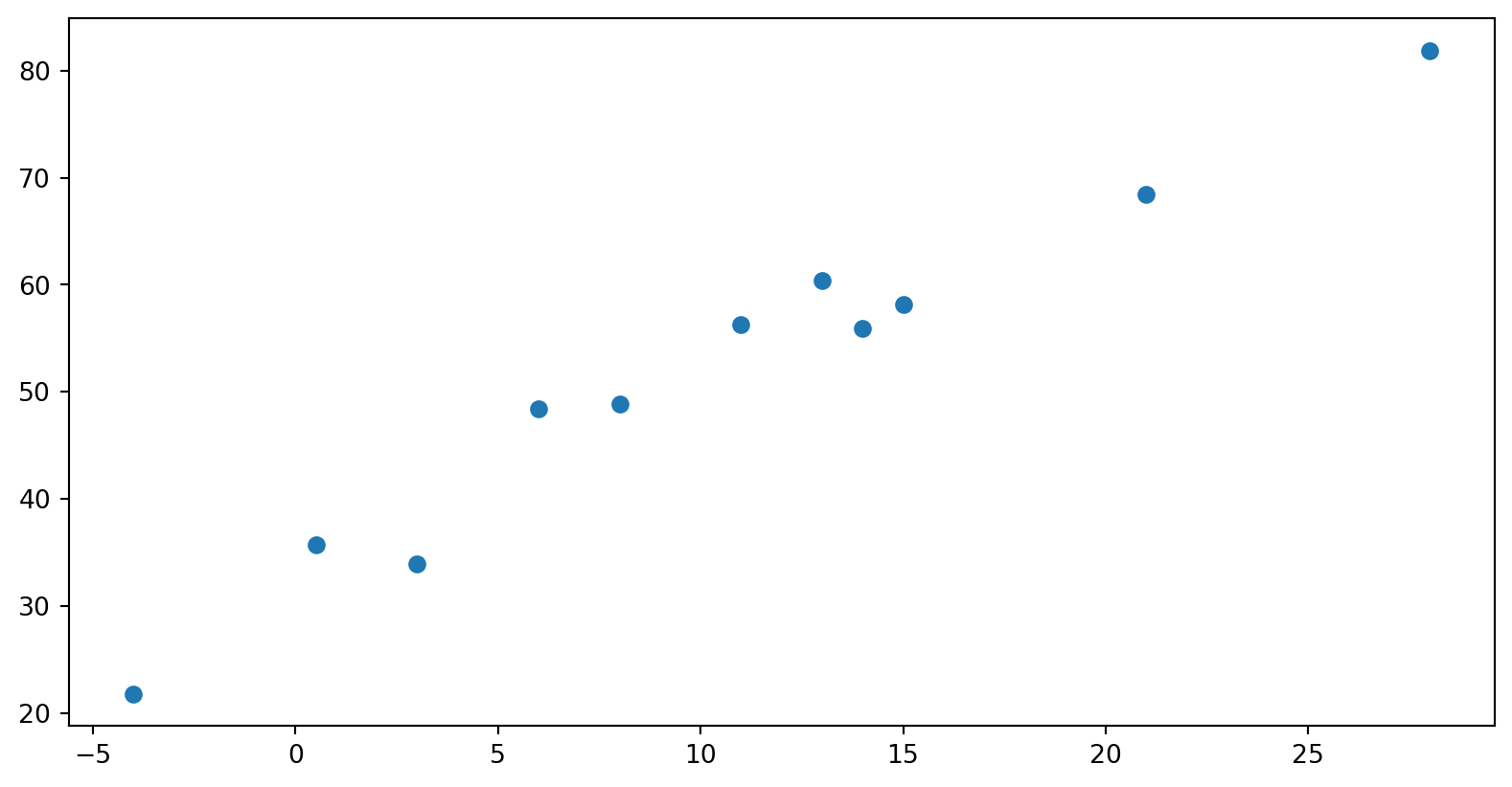
I am cold
# Input features (temperature in Celsius)
t_c = [0.5, 14.0, 15.0, 28.0, 11.0, 8.0, 3.0, -4.0, 6.0, 13.0, 21.0]
x = torch.tensor(t_c).view(-1, 1)  # Reshape to a 2D tensor with 11 rows and 1 column

# Target values (temperature in Fahrenheit)
t_u = [35.7, 55.9, 58.2, 81.9, 56.3, 48.9, 33.9, 21.8, 48.4, 60.4, 68.4]
y = torch.tensor(t_u).view(-1, 1)  # Reshape to a 2D tensor with 11 rows and 1 column
Plot it
Scale it
Think it
- Just no graceful way to do this part in R.
Also an LM
Set it up
Train it
for epoch in range(1000):
    y_pred = model(torch.tensor(x_normalized, dtype=torch.float32))
    loss = criterion(y_pred, torch.tensor(y_normalized, dtype=torch.float32))
    epoch % 100 == 0 and print(f'Epoch {epoch + 1}, Loss: {loss.item()}', model.state_dict())
    optimizer.zero_grad()
    loss.backward()
    optimizer.step()
Epoch 1, Loss: 1.4626693725585938 OrderedDict({'lin_coeffs.weight': tensor([[-0.2058]]), 'lin_coeffs.bias': tensor([0.1290])})
Epoch 101, Loss: 0.9925869107246399 OrderedDict({'lin_coeffs.weight': tensor([[0.0095]]), 'lin_coeffs.bias': tensor([0.1056])})
Epoch 201, Loss: 0.6776072978973389 OrderedDict({'lin_coeffs.weight': tensor([[0.1857]]), 'lin_coeffs.bias': tensor([0.0864])})
Epoch 301, Loss: 0.4665546119213104 OrderedDict({'lin_coeffs.weight': tensor([[0.3300]]), 'lin_coeffs.bias': tensor([0.0708])})
Epoch 401, Loss: 0.32513847947120667 OrderedDict({'lin_coeffs.weight': tensor([[0.4481]]), 'lin_coeffs.bias': tensor([0.0579])})
Epoch 501, Loss: 0.23038239777088165 OrderedDict({'lin_coeffs.weight': tensor([[0.5447]]), 'lin_coeffs.bias': tensor([0.0474])})
Epoch 601, Loss: 0.16689100861549377 OrderedDict({'lin_coeffs.weight': tensor([[0.6239]]), 'lin_coeffs.bias': tensor([0.0388])})
Epoch 701, Loss: 0.12434861809015274 OrderedDict({'lin_coeffs.weight': tensor([[0.6886]]), 'lin_coeffs.bias': tensor([0.0318])})
Epoch 801, Loss: 0.0958428829908371 OrderedDict({'lin_coeffs.weight': tensor([[0.7416]]), 'lin_coeffs.bias': tensor([0.0260])})
Epoch 901, Loss: 0.07674261927604675 OrderedDict({'lin_coeffs.weight': tensor([[0.7850]]), 'lin_coeffs.bias': tensor([0.0213])})Examine model
Penguins
Inspect Data frame
Inspect Data frame
| species | island | bill_length_mm | bill_depth_mm | flipper_length_mm | body_mass_g | sex | |
|---|---|---|---|---|---|---|---|
| 0 | Adelie | Torgersen | 39.1 | 18.7 | 181.0 | 3750.0 | Male |
| 1 | Adelie | Torgersen | 39.5 | 17.4 | 186.0 | 3800.0 | Female |
| 2 | Adelie | Torgersen | 40.3 | 18.0 | 195.0 | 3250.0 | Female |
| 4 | Adelie | Torgersen | 36.7 | 19.3 | 193.0 | 3450.0 | Female |
| 5 | Adelie | Torgersen | 39.3 | 20.6 | 190.0 | 3650.0 | Male |
We wish to label
Create a class
class PenguinDataset(Dataset):
    def __init__(self, data):
        self.X = data[['bill_length_mm', 'bill_depth_mm', 'flipper_length_mm', 'body_mass_g']].values
        self.y = data['species_encoded'].values # DONT FORGET .VALUES
        self.n_samples = len(data)

    def __getitem__(self, index):
        return torch.tensor(self.X[index], dtype=torch.float32), torch.tensor(self.y[index], dtype=torch.int64)

    def __len__(self):
        return self.n_samples
Split
train_data, test_data = train_test_split(penguins, test_size=0.2, random_state=97301)

train_dataset = PenguinDataset(train_data)
test_dataset = PenguinDataset(test_data)

train_loader = DataLoader(dataset=train_dataset, batch_size=16, shuffle=True)
test_loader = DataLoader(dataset=test_dataset, batch_size=16, shuffle=False)
Have a Look
We can ReLU
Configure the NN
Run it
Training loop
for epoch in range(10):
    model.train()
    running_loss = 0.0
    for inputs, targets in train_loader:
        optimizer.zero_grad()
        outputs = model(inputs)
        loss = criterion(outputs, targets)
        loss.backward()
        optimizer.step()
        running_loss += loss.item()
    epoch_loss = running_loss / len(train_loader)
    print(f"Epoch {epoch+1}/10, Loss: {epoch_loss:.4f}")
Epoch 1/10, Loss: 29.7547
Epoch 2/10, Loss: 9.1378
Epoch 3/10, Loss: 6.6476
Epoch 4/10, Loss: 6.5768
Epoch 5/10, Loss: 7.0012
Epoch 6/10, Loss: 4.2741
Epoch 7/10, Loss: 6.1131
Epoch 8/10, Loss: 9.5762
Epoch 9/10, Loss: 8.0600
Epoch 10/10, Loss: 6.1143Evaluation on the test set
Go line-by-line
See it
- Well that was awful. Before we fix it…
Print it
with torch.no_grad():
for i in range(3):
for batch_idx, batch in enumerate(test_loader):
outputs = model(inputs)
_, predicted = torch.max(outputs.data, 1)
print(inputs, outputs, predicted)tensor([[ 35.5000, 16.2000, 195.0000, 3350.0000],
[ 34.0000, 17.1000, 185.0000, 3400.0000],
[ 49.2000, 15.2000, 221.0000, 6300.0000]]) tensor([[12.9229, 16.4159, 16.6785],
[13.4944, 17.6571, 16.7782],
[29.4856, 42.9800, 34.9307]]) tensor([2, 1, 1])
tensor([[ 35.5000, 16.2000, 195.0000, 3350.0000],
[ 34.0000, 17.1000, 185.0000, 3400.0000],
[ 49.2000, 15.2000, 221.0000, 6300.0000]]) tensor([[12.9229, 16.4159, 16.6785],
[13.4944, 17.6571, 16.7782],
[29.4856, 42.9800, 34.9307]]) tensor([2, 1, 1])
tensor([[ 35.5000, 16.2000, 195.0000, 3350.0000],
[ 34.0000, 17.1000, 185.0000, 3400.0000],
[ 49.2000, 15.2000, 221.0000, 6300.0000]]) tensor([[12.9229, 16.4159, 16.6785],
[13.4944, 17.6571, 16.7782],
[29.4856, 42.9800, 34.9307]]) tensor([2, 1, 1])
tensor([[ 35.5000, 16.2000, 195.0000, 3350.0000],
[ 34.0000, 17.1000, 185.0000, 3400.0000],
[ 49.2000, 15.2000, 221.0000, 6300.0000]]) tensor([[12.9229, 16.4159, 16.6785],
[13.4944, 17.6571, 16.7782],
[29.4856, 42.9800, 34.9307]]) tensor([2, 1, 1])
tensor([[ 35.5000, 16.2000, 195.0000, 3350.0000],
[ 34.0000, 17.1000, 185.0000, 3400.0000],
[ 49.2000, 15.2000, 221.0000, 6300.0000]]) tensor([[12.9229, 16.4159, 16.6785],
[13.4944, 17.6571, 16.7782],
[29.4856, 42.9800, 34.9307]]) tensor([2, 1, 1])
tensor([[ 35.5000, 16.2000, 195.0000, 3350.0000],
[ 34.0000, 17.1000, 185.0000, 3400.0000],
[ 49.2000, 15.2000, 221.0000, 6300.0000]]) tensor([[12.9229, 16.4159, 16.6785],
[13.4944, 17.6571, 16.7782],
[29.4856, 42.9800, 34.9307]]) tensor([2, 1, 1])
tensor([[ 35.5000, 16.2000, 195.0000, 3350.0000],
[ 34.0000, 17.1000, 185.0000, 3400.0000],
[ 49.2000, 15.2000, 221.0000, 6300.0000]]) tensor([[12.9229, 16.4159, 16.6785],
[13.4944, 17.6571, 16.7782],
[29.4856, 42.9800, 34.9307]]) tensor([2, 1, 1])
tensor([[ 35.5000, 16.2000, 195.0000, 3350.0000],
[ 34.0000, 17.1000, 185.0000, 3400.0000],
[ 49.2000, 15.2000, 221.0000, 6300.0000]]) tensor([[12.9229, 16.4159, 16.6785],
[13.4944, 17.6571, 16.7782],
[29.4856, 42.9800, 34.9307]]) tensor([2, 1, 1])
tensor([[ 35.5000, 16.2000, 195.0000, 3350.0000],
[ 34.0000, 17.1000, 185.0000, 3400.0000],
[ 49.2000, 15.2000, 221.0000, 6300.0000]]) tensor([[12.9229, 16.4159, 16.6785],
[13.4944, 17.6571, 16.7782],
[29.4856, 42.9800, 34.9307]]) tensor([2, 1, 1])
tensor([[ 35.5000, 16.2000, 195.0000, 3350.0000],
[ 34.0000, 17.1000, 185.0000, 3400.0000],
[ 49.2000, 15.2000, 221.0000, 6300.0000]]) tensor([[12.9229, 16.4159, 16.6785],
[13.4944, 17.6571, 16.7782],
[29.4856, 42.9800, 34.9307]]) tensor([2, 1, 1])
tensor([[ 35.5000, 16.2000, 195.0000, 3350.0000],
[ 34.0000, 17.1000, 185.0000, 3400.0000],
[ 49.2000, 15.2000, 221.0000, 6300.0000]]) tensor([[12.9229, 16.4159, 16.6785],
[13.4944, 17.6571, 16.7782],
[29.4856, 42.9800, 34.9307]]) tensor([2, 1, 1])
tensor([[ 35.5000, 16.2000, 195.0000, 3350.0000],
[ 34.0000, 17.1000, 185.0000, 3400.0000],
[ 49.2000, 15.2000, 221.0000, 6300.0000]]) tensor([[12.9229, 16.4159, 16.6785],
[13.4944, 17.6571, 16.7782],
[29.4856, 42.9800, 34.9307]]) tensor([2, 1, 1])
tensor([[ 35.5000, 16.2000, 195.0000, 3350.0000],
[ 34.0000, 17.1000, 185.0000, 3400.0000],
[ 49.2000, 15.2000, 221.0000, 6300.0000]]) tensor([[12.9229, 16.4159, 16.6785],
[13.4944, 17.6571, 16.7782],
[29.4856, 42.9800, 34.9307]]) tensor([2, 1, 1])
tensor([[ 35.5000, 16.2000, 195.0000, 3350.0000],
[ 34.0000, 17.1000, 185.0000, 3400.0000],
[ 49.2000, 15.2000, 221.0000, 6300.0000]]) tensor([[12.9229, 16.4159, 16.6785],
[13.4944, 17.6571, 16.7782],
[29.4856, 42.9800, 34.9307]]) tensor([2, 1, 1])
tensor([[ 35.5000, 16.2000, 195.0000, 3350.0000],
[ 34.0000, 17.1000, 185.0000, 3400.0000],
[ 49.2000, 15.2000, 221.0000, 6300.0000]]) tensor([[12.9229, 16.4159, 16.6785],
[13.4944, 17.6571, 16.7782],
[29.4856, 42.9800, 34.9307]]) tensor([2, 1, 1])Scale it
Re-split
- Why do we have to resplit?
train_data, test_data = train_test_split(penguins, test_size=0.2, random_state=12345)
train_dataset = PenguinDataset(train_data)
test_dataset = PenguinDataset(test_data)
train_loader = DataLoader(dataset=train_dataset, batch_size=16, shuffle=True)
test_loader = DataLoader(dataset=test_dataset, batch_size=16, shuffle=False)Model Again
Learn with scaling
for epoch in range(10):
model.train()
running_loss = 0.0
for inputs, targets in train_loader:
optimizer.zero_grad()
outputs = model(inputs)
loss = criterion(outputs, targets)
loss.backward()
optimizer.step()
running_loss += loss.item()
epoch_loss = running_loss / len(train_loader)
print(f"Epoch {epoch+1}/10, Loss: {epoch_loss:.4f}")Epoch 1/10, Loss: 0.9085
Epoch 2/10, Loss: 0.7061
Epoch 3/10, Loss: 0.5581
Epoch 4/10, Loss: 0.4561
Epoch 5/10, Loss: 0.3736
Epoch 6/10, Loss: 0.3133
Epoch 7/10, Loss: 0.2612
Epoch 8/10, Loss: 0.2218
Epoch 9/10, Loss: 0.1906
Epoch 10/10, Loss: 0.1659Evaluate
Exercise
Exercise: the titanic
url = "https://web.stanford.edu/class/archive/cs/cs109/cs109.1166/stuff/titanic.csv"
titanic_df = pd.read_csv(url)
titanic_df = titanic_df.dropna() # Drop rows with missing values for simplicity
titanic_df.head()| Survived | Pclass | Name | Sex | Age | Siblings/Spouses Aboard | Parents/Children Aboard | Fare | |
|---|---|---|---|---|---|---|---|---|
| 0 | 0 | 3 | Mr. Owen Harris Braund | male | 22.0 | 1 | 0 | 7.2500 |
| 1 | 1 | 1 | Mrs. John Bradley (Florence Briggs Thayer) Cum... | female | 38.0 | 1 | 0 | 71.2833 |
| 2 | 1 | 3 | Miss. Laina Heikkinen | female | 26.0 | 0 | 0 | 7.9250 |
| 3 | 1 | 1 | Mrs. Jacques Heath (Lily May Peel) Futrelle | female | 35.0 | 1 | 0 | 53.1000 |
| 4 | 0 | 3 | Mr. William Henry Allen | male | 35.0 | 0 | 0 | 8.0500 |
Your exercise:
- Create a neural network as above to model survival on the titanic dataset.
- There are several ways to do this:
- change the size of the output layer (a simple probability, so 1)
- change the output of the final hidden layer to be a probability using nn.Sigmoid()
- change the loss criterion to be nn.BCELoss()
Notes:
- You can do this all differently: use 2 outputs (one per class), omit sigmoid and keep the same loss function, but the difference might be instructive.
- Explore variations of the model architecture (multiple hidden layers? hidden layer size? etc.)
- encourage you to print out lots of intermediate things.
- I learned a lot doing it and I bet you will too.
One solution:
One solution:
# Define a custom PyTorch dataset
class TitanicDataset(Dataset):
def __init__(self, data):
self.X = data[features].values
self.y = data[target].values
self.n_samples = len(data)
def __getitem__(self, index):
return torch.tensor(self.X[index], dtype=torch.float32), torch.tensor(self.y[index], dtype=torch.float32)
def __len__(self):
return self.n_samplesOne solution:
# Split data into train and test sets
train_data, test_data = train_test_split(titanic_df, test_size=0.2, random_state=42)
# Create PyTorch datasets and dataloaders
train_dataset = TitanicDataset(train_data)
test_dataset = TitanicDataset(test_data)
train_loader = DataLoader(dataset=train_dataset, batch_size=16, shuffle=True)
test_loader = DataLoader(dataset=test_dataset, batch_size=16, shuffle=False)One solution:
One solution:
# Define a simple neural network with one hidden layer
class SimpleNN(nn.Module):
def __init__(self, input_size, hidden_size, output_size):
super(SimpleNN, self).__init__()
self.fc1 = nn.Linear(input_size, hidden_size)
self.relu = nn.ReLU()
self.fc2 = nn.Linear(hidden_size, output_size)
self.sigmoid = nn.Sigmoid()
def forward(self, x):
out = self.fc1(x)
out = self.relu(out)
out = self.fc2(out)
out = self.sigmoid(out)
return outOne solution:
# Initialize the model, loss function, and optimizer
input_size = len(features) # Number of features
hidden_size = 64 # Size of the hidden layer
output_size = 1 # Output size (binary classification for survival)
model = SimpleNN(input_size, hidden_size, output_size)
criterion = nn.BCELoss()
optimizer = optim.SGD(model.parameters(), lr=0.001)One solution:
for epoch in range(10):
model.train()
running_loss = 0.0
for inputs, targets in train_loader:
optimizer.zero_grad()
outputs = model(inputs)
#print(outputs)
#print(targets)
#print(outputs.squeeze())
#print(outputs.shape)
#print(outputs.squeeze().shape)
loss = criterion(outputs.squeeze(), targets)
loss.backward()
optimizer.step()
running_loss += loss.item()
epoch_loss = running_loss / len(train_loader)
print(f"Epoch {epoch+1}/10, Loss: {epoch_loss:.4f}")Epoch 1/10, Loss: 0.7098
Epoch 2/10, Loss: 0.6998
Epoch 3/10, Loss: 0.6905
Epoch 4/10, Loss: 0.6832
Epoch 5/10, Loss: 0.6750
Epoch 6/10, Loss: 0.6701
Epoch 7/10, Loss: 0.6631
Epoch 8/10, Loss: 0.6592
Epoch 9/10, Loss: 0.6543
Epoch 10/10, Loss: 0.6499One solution:
model.eval()
correct = 0
total = 0
with torch.no_grad():
for inputs, targets in test_loader:
outputs = model(inputs)
predicted = torch.round(outputs)
total += targets.size(0)
correct += (predicted == targets.unsqueeze(1)).sum().item() # Ensure targets are 2D
accuracy = correct / total
print(f"Accuracy on test set: {accuracy:.2%}")Accuracy on test set: 65.17%