## Libraries Setup ```{r libs} sh <- suppressPackageStartupMessages sh(library(tidyverse)) sh(library(caret)) sh(library(tidytext)) sh(library(SnowballC)) sh(library(rpart)) # New? sh(library(randomForest)) # New? data(stop_words) sh(library(thematic)) theme_set(theme_dark()) thematic_rmd(bg = "#111", fg = "#eee", accent = "#eee") ``` ## Dataframe ```{r rds} wine <- readRDS(gzcon(url("https://cd-public.github.io/D505/dat/pinot.rds"))) names(wine)[names(wine) == 'id'] = 'id' ``` ## Wine Words ```{r setup} wine_words <- function(df, j, stem){ words <- df %>% unnest_tokens(word, description) %>% anti_join(stop_words) %>% filter(!(word %in% c("wine","pinot","vineyard"))) if(stem){ words <- words %>% mutate(word = wordStem(word)) } words %>% count(id, word) %>% group_by(id) %>% mutate(exists = (n>0)) %>% ungroup %>% group_by(word) %>% mutate(total = sum(n)) %>% filter(total > j) %>% pivot_wider(id_cols = id, names_from = word, values_from = exists, values_fill = list(exists=0)) %>% right_join(select(df,id,province)) %>% select(-id) %>% mutate(across(-province, ~replace_na(.x, F))) } ``` ## Make Wino ```{r wino} wino <- wine_words(wine, 2000, F) %>% filter(province %in% c("Oregon","California")) %>% arrange(province) wino ``` ## Algorithm 1. Select the best attribute -> $A$ 2. Assign $A$ as the decision attribute (test case) for the `NODE`. 3. For each value of $a \in A$, create a new descendant of the `NODE`. 4. Sort the training examples to the appropriate descendant node leaf. 5. If examples are perfectly classified, then `STOP` else iterate over the new leaf nodes. ## Aside: - Do we know what nodes and edges are in graph theory? - [Slides](https://cd-public.github.io/courses/old/cld24/slides/07.html#/2) ## VisualizeThis flow chart is also canonical (sincere apologies but I do not think I can alt-text this)
— lastpositivist.bsky.social (@lastpositivist.bsky.social) November 10, 2024 at 11:45 PM
[image or embed]
 ## In practice
- Where are going on vacation?
- If top 25 city in US, say city.
- Chicago
- If US but not top 25 city, say state.
- Utah
- If not US, say nation-state.
- Colombia
## Information Gain
- The *information content* of a piece of information is how "surprising" it is.
- In sports, perhaps, wins above replacement.
- In grades, perhaps, standard deviations above the mean
- In weather, perhaps, date of a rainstorm in desert vs in rainforest.
## Example
- I tell you 123456 is *not* going to win the lottery
- Very little information, and very unsurprising.
- If I tell you 123456 *will* win the lottery
- Very high information, very surprising.
## Formula
$$
I(p) = \log \left(\frac{1}{p}\right)
$$
- If $p = 1$, information is $0$
- As $p$ becomes small, $I(p)$ grows.
## Datasets
- The **entropy** of a dataset is its "average information content":
$$
{\rm Entropy}=\sum_{i=1}(p_i)\log\left(\frac{1}{p_i}\right) = \sum - p_i\log(p_i)
$$
- $p$ is the proportion of the class under consideration.
- If we have only one category, then $p_i = 1$ and entropy is 0 (no "disorder").
## Samples
- It rains 36 days per year in Phoenix.
- There are exactly 360 days per year [src](https://en.wikipedia.org/wiki/360-day_calendar)
- The "parent" node decides if a day rains, or not, and sends to other decision makers.
- $p_0 = .9$: No rain.
- $p_1 = .1$: Yes rain.
## Entropy Calculation
$$
\begin{align}
{\rm Entropy} &= \sum - p_i\log(p_i) \\
&= -.9 * \log(.9) -.1 * \log(.1)
\end{align}
$$
```{r entphx}
entropy <- -.9 * log(.9) -.1 * log(.1)
entropy
```
## Portland
- In Portland it rains 153-164 days a year.
- That is exactly half of 365
- (Don't check)
## Entropy Calculation
$$
\begin{align}
{\rm Entropy} &= \sum - p_i\log(p_i) \\
&= -.5 * \log(.5) -.5 * \log(.5) \\
&= -\log(.5)
\end{align}
$$
```{r entpdx}
entropy <- -log(.5)
entropy
```
## Surpised?
- It is more suprising to correctly guess half of days than correctly guess one tenth of days.
## Optimize
- A decision tree looks to determine the optimal binary split
- Said split maximizes *information gain*:
- The entropy of the parent, less
- The entropy of the child nodes
- Averaged
- Say probability of snow given precipitation
## Exercise
- Say we wish to classify wines by province.
- We could first see if they are fruity
- "fruit" $\in$ `desc`
- We could first see if they are tannic.
- "tanni" $\in$ `desc`
- Which is better?
## Split the data
```{r split}
wine_index <- createDataPartition(wino$province, p = 0.8, list = FALSE)
train <- wino[ wine_index, ]
test <- wino[-wine_index, ]
table(train$province)
```
## Fit a basic model
```{r rpart}
ctrl <- trainControl(method = "cv")
fit <- train(province ~ .,
data = train,
method = "rpart",
trControl = ctrl,
metric = "Kappa")
fit$finalModel
```
## Confusion Matrix
```{r}
pred <- predict(fit, newdata=test)
confusionMatrix(factor(pred), factor(test$province))
```
## Let's tune
- By setting a tune control we can try more trees.
```{r}
fit <- train(province ~ .,
data = train,
method = "rpart",
trControl = ctrl,
tuneLength = 15,
metric = "Kappa")
fit$finalModel
```
## Confusion Matrix
```{r}
pred <- predict(fit, newdata=test)
confusionMatrix(factor(pred), factor(test$province))
```
## Results
- Kappa 0.3538 -> 0.4668
- Mostly by finding more Oregon wines.
## Variable Importance
- Permutation importance
- Average split quality
```{r}
fit$finalModel$variable.importance
```
## Potential Overfitting
- Should we prune on...
- Depth?
- Class size?
- Complexity?
- Minimum Information Gain?
## Confusion Matrix
```{r}
pred <- predict(fit, newdata=test)
confusionMatrix(factor(pred), factor(test$province))
```
## Tune grids
```{r}
hyperparam_grid = expand.grid(cp = c(0, 0.01, 0.05, 0.1))
fit <- train(province ~ .,
data = train,
method = "rpart",
trControl = ctrl,
tuneGrid = hyperparam_grid,
metric = "Kappa")
fit$finalModel
```
## Confusion Matrix
```{r}
pred <- predict(fit, newdata=test)
confusionMatrix(factor(pred), factor(test$province))
```
## Exercise?
- Can you try to *overfit* as much as possible?
- Set `cp = 0`,
- Generate tons of features,
- See how out of sample performance is?
- `cp` = complexity parameter.
- Solution on next slide, more or less.
## Solution
```{r}
fit <- train(province ~ .,
data = train,
method = "rpart",
trControl = trainControl(method="none"),
tuneGrid = data.frame(cp = 0))
fit
```
## Confusion Matrix
```{r}
pred <- predict(fit, newdata=test)
confusionMatrix(factor(pred), factor(test$province))
```
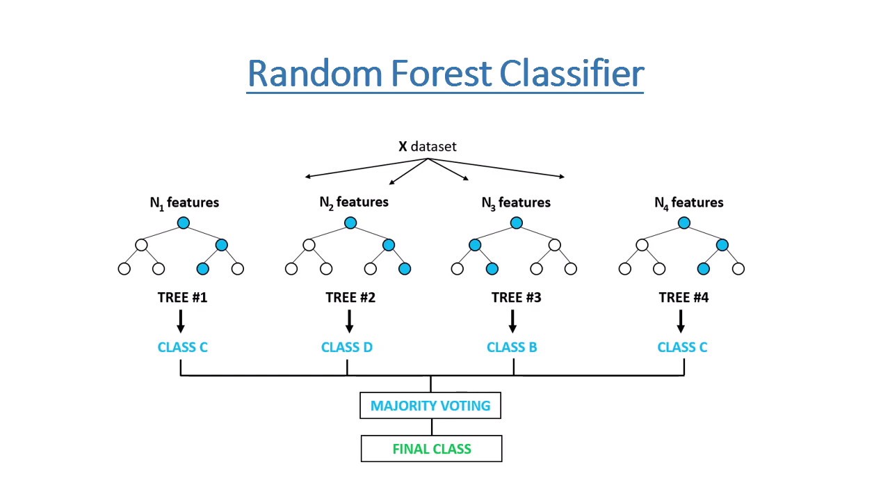
## Random Forest
```{r}
fit <- train(province ~ .,
data = train,
method = "rf",
trControl = ctrl)
fit
```
## Confusion Matrix
```{r}
pred <- predict(fit, newdata=test)
confusionMatrix(factor(pred),factor(test$province))
```
## Pros
- Easy to use and understand.
- Can handle both categorical and numerical data.
- Resistant to outliers, hence require little data preprocessing.
- New features can be easily added.
- Can be used to build larger classifiers by using ensemble methods.
## Cons
- Prone to overfitting.
- Require some kind of measurement as to how well they are doing.
- Need to be careful with parameter tuning.
- Can create biased learned trees if some classes dominate.
# Group Work
## In practice
- Where are going on vacation?
- If top 25 city in US, say city.
- Chicago
- If US but not top 25 city, say state.
- Utah
- If not US, say nation-state.
- Colombia
## Information Gain
- The *information content* of a piece of information is how "surprising" it is.
- In sports, perhaps, wins above replacement.
- In grades, perhaps, standard deviations above the mean
- In weather, perhaps, date of a rainstorm in desert vs in rainforest.
## Example
- I tell you 123456 is *not* going to win the lottery
- Very little information, and very unsurprising.
- If I tell you 123456 *will* win the lottery
- Very high information, very surprising.
## Formula
$$
I(p) = \log \left(\frac{1}{p}\right)
$$
- If $p = 1$, information is $0$
- As $p$ becomes small, $I(p)$ grows.
## Datasets
- The **entropy** of a dataset is its "average information content":
$$
{\rm Entropy}=\sum_{i=1}(p_i)\log\left(\frac{1}{p_i}\right) = \sum - p_i\log(p_i)
$$
- $p$ is the proportion of the class under consideration.
- If we have only one category, then $p_i = 1$ and entropy is 0 (no "disorder").
## Samples
- It rains 36 days per year in Phoenix.
- There are exactly 360 days per year [src](https://en.wikipedia.org/wiki/360-day_calendar)
- The "parent" node decides if a day rains, or not, and sends to other decision makers.
- $p_0 = .9$: No rain.
- $p_1 = .1$: Yes rain.
## Entropy Calculation
$$
\begin{align}
{\rm Entropy} &= \sum - p_i\log(p_i) \\
&= -.9 * \log(.9) -.1 * \log(.1)
\end{align}
$$
```{r entphx}
entropy <- -.9 * log(.9) -.1 * log(.1)
entropy
```
## Portland
- In Portland it rains 153-164 days a year.
- That is exactly half of 365
- (Don't check)
## Entropy Calculation
$$
\begin{align}
{\rm Entropy} &= \sum - p_i\log(p_i) \\
&= -.5 * \log(.5) -.5 * \log(.5) \\
&= -\log(.5)
\end{align}
$$
```{r entpdx}
entropy <- -log(.5)
entropy
```
## Surpised?
- It is more suprising to correctly guess half of days than correctly guess one tenth of days.
## Optimize
- A decision tree looks to determine the optimal binary split
- Said split maximizes *information gain*:
- The entropy of the parent, less
- The entropy of the child nodes
- Averaged
- Say probability of snow given precipitation
## Exercise
- Say we wish to classify wines by province.
- We could first see if they are fruity
- "fruit" $\in$ `desc`
- We could first see if they are tannic.
- "tanni" $\in$ `desc`
- Which is better?
## Split the data
```{r split}
wine_index <- createDataPartition(wino$province, p = 0.8, list = FALSE)
train <- wino[ wine_index, ]
test <- wino[-wine_index, ]
table(train$province)
```
## Fit a basic model
```{r rpart}
ctrl <- trainControl(method = "cv")
fit <- train(province ~ .,
data = train,
method = "rpart",
trControl = ctrl,
metric = "Kappa")
fit$finalModel
```
## Confusion Matrix
```{r}
pred <- predict(fit, newdata=test)
confusionMatrix(factor(pred), factor(test$province))
```
## Let's tune
- By setting a tune control we can try more trees.
```{r}
fit <- train(province ~ .,
data = train,
method = "rpart",
trControl = ctrl,
tuneLength = 15,
metric = "Kappa")
fit$finalModel
```
## Confusion Matrix
```{r}
pred <- predict(fit, newdata=test)
confusionMatrix(factor(pred), factor(test$province))
```
## Results
- Kappa 0.3538 -> 0.4668
- Mostly by finding more Oregon wines.
## Variable Importance
- Permutation importance
- Average split quality
```{r}
fit$finalModel$variable.importance
```
## Potential Overfitting
- Should we prune on...
- Depth?
- Class size?
- Complexity?
- Minimum Information Gain?
## Confusion Matrix
```{r}
pred <- predict(fit, newdata=test)
confusionMatrix(factor(pred), factor(test$province))
```
## Tune grids
```{r}
hyperparam_grid = expand.grid(cp = c(0, 0.01, 0.05, 0.1))
fit <- train(province ~ .,
data = train,
method = "rpart",
trControl = ctrl,
tuneGrid = hyperparam_grid,
metric = "Kappa")
fit$finalModel
```
## Confusion Matrix
```{r}
pred <- predict(fit, newdata=test)
confusionMatrix(factor(pred), factor(test$province))
```
## Exercise?
- Can you try to *overfit* as much as possible?
- Set `cp = 0`,
- Generate tons of features,
- See how out of sample performance is?
- `cp` = complexity parameter.
- Solution on next slide, more or less.
## Solution
```{r}
fit <- train(province ~ .,
data = train,
method = "rpart",
trControl = trainControl(method="none"),
tuneGrid = data.frame(cp = 0))
fit
```
## Confusion Matrix
```{r}
pred <- predict(fit, newdata=test)
confusionMatrix(factor(pred), factor(test$province))
```
## Random Forest

```{r}
fit <- train(province ~ .,
data = train,
method = "rf",
trControl = ctrl)
fit
```
## Confusion Matrix
```{r}
pred <- predict(fit, newdata=test)
confusionMatrix(factor(pred),factor(test$province))
```
## Pros
- Easy to use and understand.
- Can handle both categorical and numerical data.
- Resistant to outliers, hence require little data preprocessing.
- New features can be easily added.
- Can be used to build larger classifiers by using ensemble methods.
## Cons
- Prone to overfitting.
- Require some kind of measurement as to how well they are doing.
- Need to be careful with parameter tuning.
- Can create biased learned trees if some classes dominate.
# Group Work