SciPy

Scientific Computing

Prof. Calvin

Why SciPy?

What is SciPy?

SciPy (pronounced “Sigh Pie”) is an open-source software for mathematics, science, and engineering.

Scientific Python
Basically a NumPy extension.

Why SciPy

Most popular scientific computing platform in the world.
Basis of scikit-learn, the most popular machine learning platform in the world.
Extremely rigorous - most functions and documentation come with academic citations.

Why not SciPy

SciPy for statistics has basically one challenger (statsmodels, which is great).
Sometimes SciPy is too “heavyweight” and NumPy would be sufficient.
As a rule, I tend to use NumPy for easy things and scikit-learn for hard things, and don’t use SciPy for much.

Relevance

This is a scientific computing course!
We’ll do a bit of signal processing and interpolation.

Credits

SciPy is a big, complex library with many components.
I used each of:
- The User Guide
- The API reference
  - API is “application program interface” - a description of the functions in SciPy by their arguments and return values.
- The Cookbook which may be unofficial.

Install

pip again

Just like NumPy, Matplotlib is a Python package which we install via pip

python3 -m pip install scipy

That might take a moment, when it does we can check it worked!

Verify

We can quickly verify installation and introduce some conventions.
Open up Python and import the libraries:

import numpy as np
import matplotlib.pyplot as plt
import scipy

print(scipy.__version__)

1.14.1

Other Installs

Motivation

I thought it would be fun to do some signal processing on a recognizable data set:
PSY - GANGNAM STYLE(강남스타일) M/V

YouTube

STOP

Instructor’s note: Do not click this link while streaming.

Problem Statement

SciPy has the ability to read some filetypes but not others.
- Can read: “.wav” Waveform Audio File Format.
- Can’t read: YouTube urls
We use Python package yt-dlp to download from YouTube.
We use non-Python package ffmpeg to translate .mp4 files to .wav
We use VideoLAN VLC Media Player to play the .wav files.

Note

You do not need to download any of these.
Here is the .wav:
Here is a link:
- psy.wav

yt-dlp

While I don’t think you need it for anything, I installed yt-dlp as follows, from the shell:

python -m pip install yt-dlp

ffmpeg

I believe this is the best place to download ffmpeg for Windows and MacOS.
https://www.ffmpeg.org/download.html
I used it on Ubuntu Linux and did not attempt and Windows or MacOS install.

Download

Both yt-dlp and ffmpeg are command line utilites (like Python, Neovim, or ls).
I didn’t actually ever use ffmpeg directly, it is just used by yt-dlp.
Given the url, I used the following shell command:

yt-dlp -x --audio-format wav https://www.youtube.com/watch?v=9bZkp7q19f0 -o psy.wav

This tells yt-dlp to go to the url, download to video, convert it to a .wav, and save it as “psy.wav”

VLC

I highly recommend having VLC installed.
https://www.videolan.org/vlc/#download

curl

As an alternative, you can curl the file.
- Just the one I extracted.
The curl shell command downloads files from urls.
- Can also be used to get “.csv” files for pandas!

curl https://github.com/cd-public/scicom/raw/refs/heads/main/qmd/src/psy.wav -o psy.wav

This directs the command line to download the file from the url and save it locally as “psy.wav”

`scipy.io`

wavfile

To load a wavfile into SciPy, it is a simple matter.
But first, we note one difference:
- With NumPy, we imported as np
- With pandas, we import as pd
With Matplotlib, we imported Matplotlib “dot” something - pyplot
- The “Python interface”

SciPy Modules

SciPy is composed of many modules
matplotlib.pyplot is a previous example of a module.
For example:
- scipy.io includes ways to read files.
- scipy.fft does Fast Fourier Transforms.
- scipy.stats does statistics.

Load “psy.wav”

We will load a sound file as an np.array.

rate, data = scipy.io.wavfile.read("psy.wav")

This may look odd!

Multiple return

This uses a slightly advanced Python topic of “multiple return”.

def roots(x):
    root = np.sqrt(x)
    return -root, root

Python can return multiple comma-separated values from a function.

neg, pos = roots(25)
[neg, pos]

[np.float64(-5.0), np.float64(5.0)]

We can “unpack” the multiple values by providing comma separated variable names.

Aside: Tuples

These multiple returns are just tuples.
- The things that are like lists, but not exactly.

both = roots(64)
type(both)

tuple

We can also use indexing to see individual elements of a tuple.

both[0]

np.float64(-8.0)

vs. Lists

The only difference compared to lists is updates.
In a list, we can change an element with its index:

color_lst = ["red", "orange", "yellow", "green", "blue", "indigo", "violet"]
color_lst[-1] = "purple"
color_lst

['red', 'orange', 'yellow', 'green', 'blue', 'indigo', 'purple']

Aside: Errors

Attempting updates to a tuple will error.
Thus far we have avoided showing example code that won’t work.
We can use try and except (like if and else) on erroneous code.

color_tup = tuple(color_lst)
try:
    color_tup[-1] = "violet"
except:
    print("Tuples can't do that.")

Tuples can't do that.

Reading files

Try/except is very handy when reading files.
A lot of files I try to read are garbled and can’t be read.
Using try and except prevents Python errors.
- More useful in big scripts than single-line things.

Example

While making these slides, I tried the curl command to get “psy.wav” while (unbeknownst to me) my internet was spotty.
I got a file named “psy.wav” that was of size 0
Unsurprisingly, opening it with SciPy led to an error.
This happens all the time!

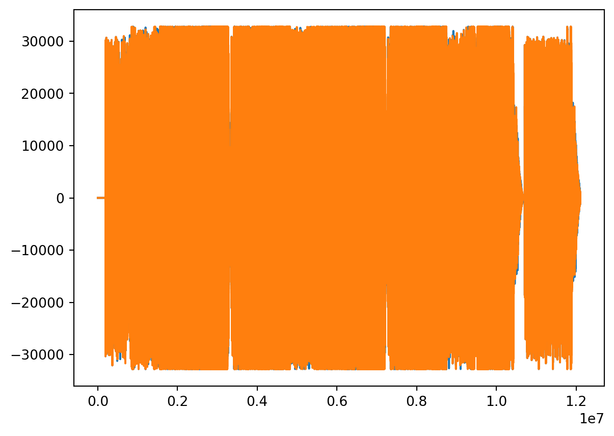
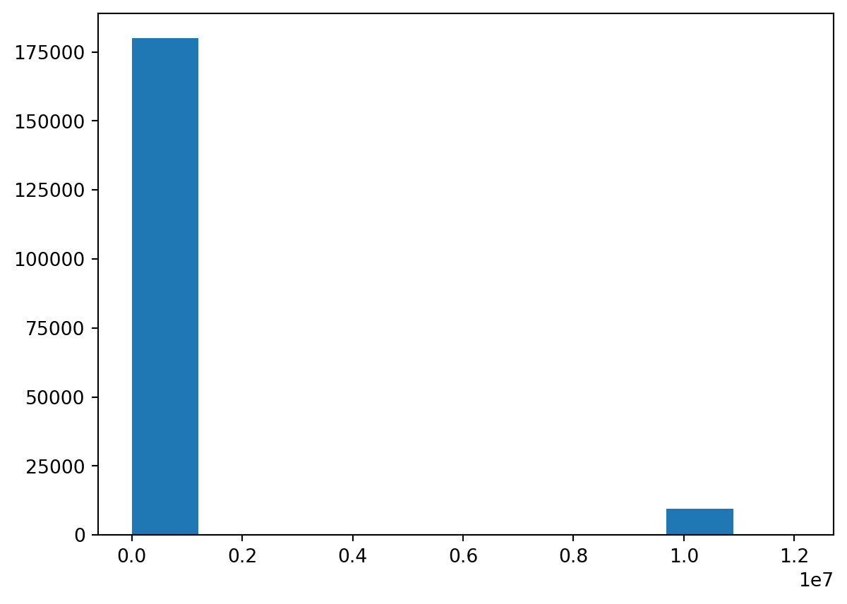
Data

Back to our .wav file.
Let’s look at that data!

data[:10]

array([[0, 0],
       [0, 0],
       [0, 0],
       [0, 0],
       [0, 0],
       [0, 0],
       [0, 0],
       [0, 0],
       [0, 0],
       [0, 0]], dtype=int16)

Rate

rate

You may have listened to the file (or not).
Audio doesn’t come in for about 4 seconds.
The song ends and there’s a kind of “outro”.
We can see these on the plot.
But that explains the zeros.

Plot

plt.plot(data)

Back to Data

Given the rate, we can look at values ever rate amount of time.
I bet it’s seconds, so we’ll see 3 or 4 zero-only then some non-zero.

data[:rate*10:rate]

array([[     0,      0],
       [     0,      0],
       [     0,      0],
       [     0,      0],
       [    -2,      3],
       [-13903, -13896],
       [ 12440,  12442],
       [  6053,   6051],
       [  5888,   5888],
       [    53,     52]], dtype=int16)

Why pairs?

Those two values may look initially suspicious, then I remembered.
Many mammals, including some assistant professors of computer science, have two ears!
This is a stereo file - the pairs are for each of two speakers.

Test it

Don’t believe me?
Let’s split into a “left” and “right” file.
We needn’t necessarily get the labels right, but these are simply NumPy operations.
Then listen!

Transpose

Remember .transpose?
It will take an array of pairs and make a pair of arrays.

tpose = data.transpose()
tpose[0][:rate*10:rate]

array([     0,      0,      0,      0,     -2, -13903,  12440,   6053,
         5888,     53], dtype=int16)

Split

I will arbitrarily call one “left” and one “rite” (not “right” because we don’t know if we’re right).

left = tpose[0]
rite = tpose[1]

Zeros

We’ll also make a zero-only array of the same length.

# We note the "dtype" was "int16" so we do the same.
# We do have to be clear it's NumPy int16 though!
zero = np.zeros(len(left),dtype=np.int16)

Combine

We can make left-only and rite-only arrays via:
- Combine
- Transpose

left_only = np.array([left,zero]).transpose()
left_only[:rate*10:rate]

array([[     0,      0],
       [     0,      0],
       [     0,      0],
       [     0,      0],
       [    -2,      0],
       [-13903,      0],
       [ 12440,      0],
       [  6053,      0],
       [  5888,      0],
       [    53,      0]], dtype=int16)

rite_only = np.array([zero,rite]).transpose()
rite_only[:rate*10:rate]

array([[     0,      0],
       [     0,      0],
       [     0,      0],
       [     0,      0],
       [     0,      3],
       [     0, -13896],
       [     0,  12442],
       [     0,   6051],
       [     0,   5888],
       [     0,     52]], dtype=int16)

Save

Let’s write/save both then give ’um a listen.

scipy.io.wavfile.write("left.wav", rate, left_only)

scipy.io.wavfile.write("rite.wav", rate, rite_only)

Listen

Let’s write/save both then give ’um a listen.

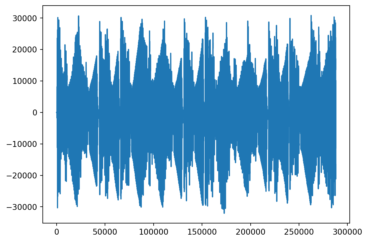
Noise

Noise Reduction

In a way, all sound is noise.
Let’s try and isolate the vocals and music, regarding the other variously as noise at various points.
First identify where vocals come in.
To me, 0:04 to 0:09 seems instrumental.

View it

Look for patterns

snip = left[4*rate:10*rate]
plt.plot(snip)

Repeats?

Looks like volume cuts low on a repeated pattern.
Maybe we can isolate that pattern.
Let’s:
- Pick a range
- Find a minimal value
- Find where that value occurs.

low_val = min(snip)
low_val

np.int16(-32071)

Whoops!

Oh we need to use absolute value.
No worries!

low_val = min(np.absolute(snip))
low_val

np.int16(0)

Where?

Use np.where to find where the low values occur.
- We used with pandas

lows = np.where(snip == 0)
lows

(array([    13,     14,     18,     20,     31,     39,     44,    126,
           127,    136,    137,    138,    148,    155,    157,    174,
           176,    193,    197,    202,    219,    221,    222,    223,
           231,    232,    262,    268,    317,    383,    405,    430,
         13580,  25648,  26839,  28676,  29655,  64732, 131187, 131204,
        153051, 210217, 216983, 271632, 278282]),)

Patterns

Maybe there’s something repeating on a periodicity of like… 65k?

# We note that the result was enclosed in () so we get the [0] of it.
lows = lows[0]
# Then proceed
lows = lows[np.where(lows > 500)]
lows

array([ 13580,  25648,  26839,  28676,  29655,  64732, 131187, 131204,
       153051, 210217, 216983, 271632, 278282])

Visualize

Let’s just plot the place the minimum occurs.

_ = plt.hist(lows)

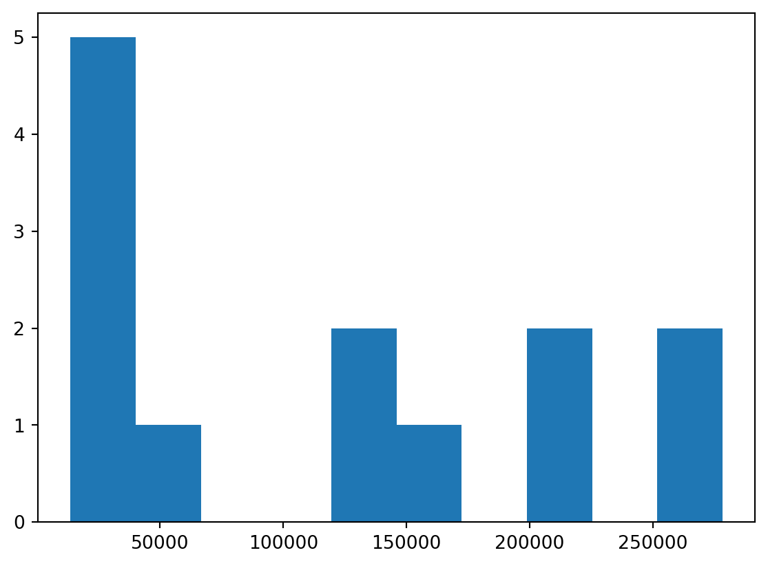
More Bins

Hard to see, we increase the “bin” count.

_ = plt.hist(lows, 100)

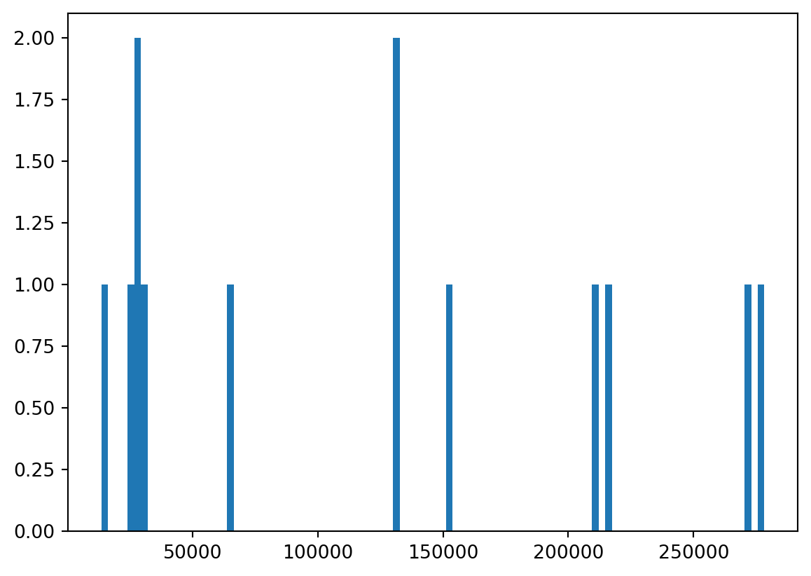
A Pattern?

_ = plt.hist(np.where(left == 0))

Only before vocals enter?

Isolate

Let’s see if we can isolate a motif.
We’ll take the first zero past.
I hear about two repeats on this portion, so we’ll take a zero in the middle.

np.where(snip == 0)

(array([    13,     14,     18,     20,     31,     39,     44,    126,
           127,    136,    137,    138,    148,    155,    157,    174,
           176,    193,    197,    202,    219,    221,    222,    223,
           231,    232,    262,    268,    317,    383,    405,    430,
         13580,  25648,  26839,  28676,  29655,  64732, 131187, 131204,
        153051, 210217, 216983, 271632, 278282]),)

Motif

stereo = np.array([snip,snip]).transpose()
motif = stereo[13580:131204]
scipy.io.wavfile.write("motif.wav", rate, motif)
# os.system("open motif.wav") # After import, if you have VLC, on MacOS

other = stereo[13580:271632]
scipy.io.wavfile.write("other.wav", rate, other)

scipy.io.wavfile.write("motifs.wav", rate, np.concatenate([motif,motif,motif]))
scipy.io.wavfile.write("others.wav", rate, np.concatenate([other,other,other]))

You can go become a dj, or…

FFT

The actual correct way to do this is with a SciPy FFT:
- Fast Fourier Transform
And with a NumPy stride:
- Stride Tricks
Which is probably a bit much for now.

Stats

Regression

One of the most used computation techniques is regression.
It is used throughout the sciences, but most commonly in econometrics.
In my my undergraduate economics class, I had a homework assignment to “prove” that raising minimum wage increases unemployment.
- It doesn’t, but that isn’t relevant here.

The Data

I usually get economic data from the “St. Louis Fed” which has a data portal called “FRED”.
- Minimum wage FEDMINNFRWG
- Unemployment rage UNRATE
- Inflation CPIAUCSL

curl

It is actually possible to curl these but you probably have to navigate the websites to find the urls regardless.
I retrieved these manually on MS Windows on 31 May 2025 at 7:33 PM PT.

curl https://github.com/cd-public/scicom/raw/refs/heads/main/qmd/src/FEMINNFRWG.csv -o FEDMINNFRWG.csv
curl https://github.com/cd-public/scicom/raw/refs/heads/main/qmd/src/UNRATE.csv-o UNRATE.csv
curl https://github.com/cd-public/scicom/raw/refs/heads/main/qmd/src/CPIAUCSL.csv -o CPIAUCSL.csv

Within Python

You can of course also get these with out leaving Python.
Given some url with Python
- url = "https://..."
You can of course also:
- pandas pd.read_csv(url)
- “os” os.system("curl " + url + " -o name.csv")

How I did it

import pandas as pd

minwage = pd.read_csv("https://github.com/cd-public/scicom/raw/refs/heads/main/qmd/src/FEDMINNFRWG.csv")
unemploy = pd.read_csv("https://github.com/cd-public/scicom/raw/refs/heads/main/qmd/src/UNRATE.csv")
inflate = pd.read_csv("https://github.com/cd-public/scicom/raw/refs/heads/main/qmd/src/CPIAUCSL.csv")
inflate

	observation_date	CPIAUCSL
0	1947-01-01	21.480
1	1947-02-01	21.620
2	1947-03-01	22.000
3	1947-04-01	22.000
4	1947-05-01	21.950
...	...	...
935	2024-12-01	317.603
936	2025-01-01	319.086
937	2025-02-01	319.775
938	2025-03-01	319.615
939	2025-04-01	320.321

940 rows × 2 columns

Check Columns

minwage.columns

Index(['observation_date', 'FEDMINNFRWG'], dtype='object')

unemploy.columns

Index(['observation_date', 'UNRATE'], dtype='object')

inflate.columns

Index(['observation_date', 'CPIAUCSL'], dtype='object')

Merge

This is suitable for a merge.
Alternatively, set date as index then join.

df = minwage.merge(unemploy).merge(inflate)
df = df.drop(columns=["observation_date"])
df[:3]

	FEDMINNFRWG	UNRATE	CPIAUCSL
0	0.4	3.4	23.68
1	0.4	3.8	23.67
2	0.4	4.0	23.50

Adjustments

Unemployment rate is rate.
Minimum wage is a nominal value (e.g. it’s units are ill-defined).
Inflation is an index of wage units.
We can divide wage by inflation to get a “real wage”.

# I made so many types here.
# In a pinch use df[df.columns[0]]
df["REAL"] = df["FEDMINNFRWG"] / df["CPIAUCSL"]

Percent Change

We measure percent change in real wages.
- We use pandas .pct_change()
  - It’s recommend by SciPy
- We drop the row 0 which has no percent change.
  - Drop rows by index, vs column=<name>
- We drop an undefined (“NaN”) values

df["REALPCT"] = df["REAL"].pct_change()
df.drop(0)
df = df.dropna()

Unemployment

Oh we should probably take a percentage change in unemployment as well.

df["UNRATE"] = df["UNRATE"].pct_change()

Look at it

plt.xlabel("REALPCT")
plt.ylabel("UNRATE")
_ = plt.scatter(df["REALPCT"],df["UNRATE"])

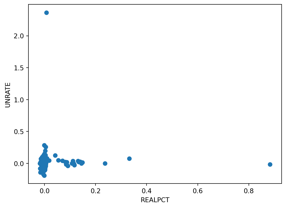
Linear Regression

The standard measure of statistical significance.
We are assuming linearity, but it is already a comparison between rates.
For more, study statistics!

from scipy import stats

`linregress`

res = stats.linregress(df["REALPCT"],df["UNRATE"])
print(res)

LinregressResult(slope=np.float64(nan), intercept=np.float64(nan), rvalue=np.float64(nan), pvalue=np.float64(nan), stderr=np.float64(nan), intercept_stderr=np.float64(nan))

Tada!

Raising minimum wage doesn’t predictable impact unemployment.

Exercise

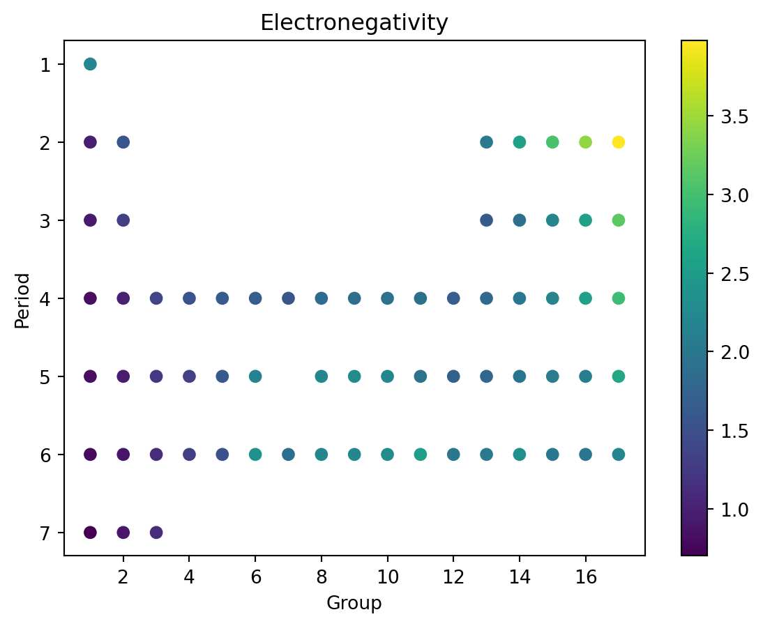
Technetium

We recall the periodic table data

df = pd.read_csv("https://gist.githubusercontent.com/GoodmanSciences/c2dd862cd38f21b0ad36b8f96b4bf1ee/raw/1d92663004489a5b6926e944c1b3d9ec5c40900e/Periodic%2520Table%2520of%2520Elements.csv")
df[::30]

	AtomicNumber	Element	Symbol	AtomicMass	NumberofNeutrons	NumberofProtons	NumberofElectrons	Period	Group	Phase	...	FirstIonization	Density	MeltingPoint	BoilingPoint	NumberOfIsotopes	Discoverer	Year	SpecificHeat	NumberofShells	NumberofValence
0	1	Hydrogen	H	1.007	0	1	1	1	1.0	gas	...	13.5984	0.00009	14.175	20.28	3.0	Cavendish	1766.0	14.304	1	1.0
30	31	Gallium	Ga	69.723	39	31	31	4	13.0	solid	...	5.9993	5.91000	302.910	2477.00	14.0	de Boisbaudran	1875.0	0.371	4	3.0
60	61	Promethium	Pm	145.000	84	61	61	6	NaN	artificial	...	5.5820	7.26000	1204.150	3273.00	14.0	Marinsky et al.	1945.0	NaN	6	NaN
90	91	Protactinium	Pa	231.036	140	91	91	7	NaN	solid	...	5.8900	15.40000	1873.150	4300.00	14.0	Hahn and Meitner	1917.0	NaN	7	NaN

4 rows × 28 columns

Interpolation

When first setting out the table, a number of elements had not yet been “observed”
- That is, no one determined their chemical properties while away they were an element.
Some certainly were never observed, namely technetium (Tc, 43) which does not exist in nature.
However, the layout of the table allowed scientists to predict properties of technetium

Extract

We will:
- Set aside technetium in a variable to check our predictions against.
- Remove the “transuranic” elements which were also not yet observed.

df = df.iloc[:91]
Tc = df.iloc[42]
df = df.drop(42)
Tc

AtomicNumber                        43
Element                     Technetium
Symbol                              Tc
AtomicMass                        98.0
NumberofNeutrons                    55
NumberofProtons                     43
NumberofElectrons                   43
Period                               5
Group                              7.0
Phase                       artificial
Radioactive                        yes
Natural                            NaN
Metal                              yes
Nonmetal                           NaN
Metalloid                          NaN
Type                  Transition Metal
AtomicRadius                       2.0
Electronegativity                  1.9
FirstIonization                   7.28
Density                           11.5
MeltingPoint                   2473.15
BoilingPoint                    5150.0
NumberOfIsotopes                  23.0
Discoverer           Perrier and Segr�
Year                            1937.0
SpecificHeat                       NaN
NumberofShells                       5
NumberofValence                    NaN
Name: 42, dtype: object

Import

To save some typing, we’ll import it directly.

from scipy.interpolate import LinearNDInterpolator

Data

We recall electronegativity.

Code

# Plot
plt.scatter(
    x=df["Group"],
    y=df["Period"],
    c=df["Electronegativity"]
)
plt.gca().invert_yaxis()
# Label
plt.title("Electronegativity")
plt.xlabel("Group")
plt.ylabel("Period")
_ = plt.colorbar()

Reference

The documentation we’re following is here

Code

from scipy.interpolate import LinearNDInterpolator
import numpy as np
import matplotlib.pyplot as plt
rng = np.random.default_rng()
x = rng.random(10) - 0.5
y = rng.random(10) - 0.5
z = np.hypot(x, y)
X = np.linspace(min(x), max(x))
Y = np.linspace(min(y), max(y))
X, Y = np.meshgrid(X, Y)  # 2D grid for interpolation
interp = LinearNDInterpolator(list(zip(x, y)), z)
Z = interp(X, Y)
plt.pcolormesh(X, Y, Z, shading='auto')
plt.plot(x, y, "ok", label="input point")
plt.legend()
plt.colorbar()
plt.axis("equal")
plt.show()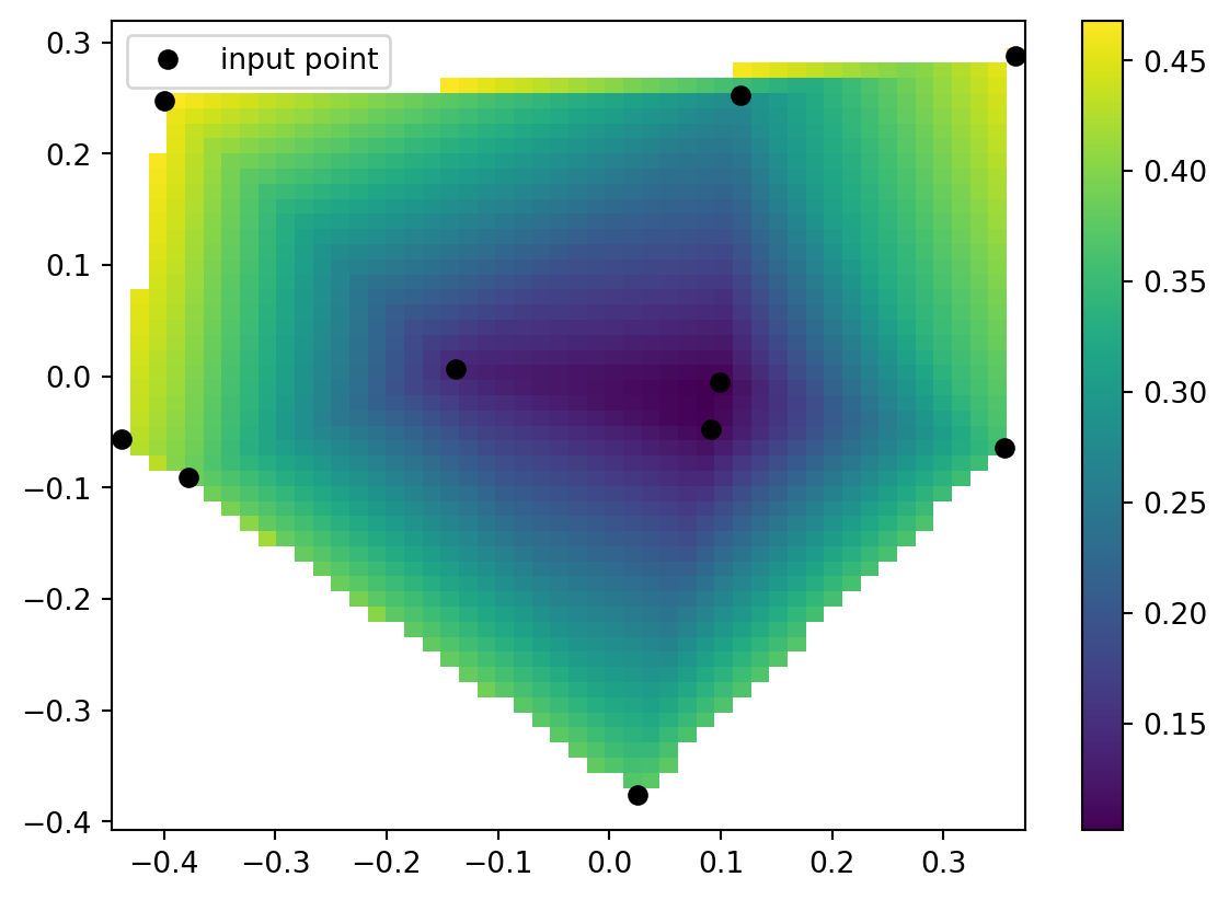

Working df

We need a df to work with.
We need only Group, Period, Electronegativity
We must not have any invalid entries.
We modify df to have only these 3 values, then .dropna()

df = df[["Group", "Period", "Electronegativity"]]
df = df.dropna()

X

We will:
- Determine the input x values.
- We call this X (capitalized) to denote it is a vector or array.
We used “Group” for x.

X = df["Group"]
X[::20]

0      1.0
23     6.0
45    10.0
80    13.0
Name: Group, dtype: float64

Y

We will:
- Determine the input x values.
- We call this Y (capitalized) to denote it is a vector or array.
We used “Period” for y.

Y = df["Period"]
Y[::20]

0     1
23    4
45    5
80    6
Name: Period, dtype: int64

2D

We will:
- Create the 2D space given X and Y
- This is a “column stack”

arr2d = np.column_stack((X,Y))
arr2d[::20]

array([[ 1.,  1.],
       [ 6.,  4.],
       [10.,  5.],
       [13.,  6.]])

Z

We will:
- Provide known output values as Z

Z = df["Electronegativity"]
Z

0     2.20
2     0.98
3     1.57
4     2.04
5     2.55
      ... 
83    2.00
84    2.20
86    0.70
87    0.90
88    1.10
Name: Electronegativity, Length: 68, dtype: float64

SciPy

Back to SciPy!
- Use LinearNDInterpolar
It basically makes a function that theoretically described electronegativity.

Stop!

Note

We are about to, essentially, conduct an experiment!
We should make a hypothesis first, then test it.
First, naively predict Tc’s electronegativity, and write down your guess!

The next slides have my guess, but you should make your own guess first!

My Guess

I took the electronegativity of Tc’s neighbors vertically and horizontally.

Tc

AtomicNumber                        43
Element                     Technetium
Symbol                              Tc
AtomicMass                        98.0
NumberofNeutrons                    55
NumberofProtons                     43
NumberofElectrons                   43
Period                               5
Group                              7.0
Phase                       artificial
Radioactive                        yes
Natural                            NaN
Metal                              yes
Nonmetal                           NaN
Metalloid                          NaN
Type                  Transition Metal
AtomicRadius                       2.0
Electronegativity                  1.9
FirstIonization                   7.28
Density                           11.5
MeltingPoint                   2473.15
BoilingPoint                    5150.0
NumberOfIsotopes                  23.0
Discoverer           Perrier and Segr�
Year                            1937.0
SpecificHeat                       NaN
NumberofShells                       5
NumberofValence                    NaN
Name: 42, dtype: object

One Way

Tc is group 7 and period 5, so, perhaps…

# DataFrame "vertical horizontal neighbors"
vh = df[df["Group"] >= 6]
vh = vh[vh["Group"] <= 8]
vh = vh[vh["Period"] >= 4]
vh = vh[vh["Period"] <= 6]
vh

	Group	Period	Electronegativity
23	6.0	4	1.66
24	7.0	4	1.55
25	8.0	4	1.83
41	6.0	5	2.16
43	8.0	5	2.20
73	6.0	6	2.36
74	7.0	6	1.90
75	8.0	6	2.20

Aside: Boolean Index

The previous example was not graceful.
We can use Boolean Indexing
The range detection method used earlier in piecewise.py doesn’t work on arrays unfortunately.
But (array < value) & (array > value) works.

Aside: Example

vh = df[(df["Group"] >= 6) & (df["Group"] <= 8) & (df["Period"] >= 4) & (df["Period"] <= 6)]
vh

	Group	Period	Electronegativity
23	6.0	4	1.66
24	7.0	4	1.55
25	8.0	4	1.83
41	6.0	5	2.16
43	8.0	5	2.20
73	6.0	6	2.36
74	7.0	6	1.90
75	8.0	6	2.20

Aside: Immediate Neighbor

It actually probably makes more sense to take
- The sum, of
- The absolute values, of
- The differences, between
  - Tc’s group and period, and
  - The tested row’s group and period.

Immediate Example

close = df[(abs(df["Group"] - 7) + abs(df["Period"] - 5)) < 2]
close

	Group	Period	Electronegativity
24	7.0	4	1.55
41	6.0	5	2.16
43	8.0	5	2.20
74	7.0	6	1.90

My Estimate:

After picking what I thought was things near Tc that should cancel out each other’s distance, I calculate their mean.

my_pred = close["Electronegativity"].mean()
my_pred

np.float64(1.9525000000000001)

This is my naive prediction.
Now I interpolate.

Interpolate

LinearNDInterpolator takes an array of known inputs and an array of known outputs and returns a function that it thinks describes the relationship.
“Thinks” being a vague term here to convey a sense of learning or prediction or estimation.

f = LinearNDInterpolator(arr2d, Z)
scipy_pred = f(7,5)
[scipy_pred, my_pred, Tc["Electronegativity"]]

[array(1.725), np.float64(1.9525000000000001), np.float64(1.9)]

Exercise

Predict using your own methods the density of Tc.
Interpolate using SciPy the density of Tc.

Solution

Code

df = pd.read_csv("https://gist.githubusercontent.com/GoodmanSciences/c2dd862cd38f21b0ad36b8f96b4bf1ee/raw/1d92663004489a5b6926e944c1b3d9ec5c40900e/Periodic%2520Table%2520of%2520Elements.csv")
df.drop(42)
df = df[["Group", "Period", "Density"]]
df = df.dropna()
f = LinearNDInterpolator(np.column_stack((df["Group"],df["Period"])), df["Density"])
me = df[(abs(df["Group"] - 7) + abs(df["Period"] - 5)) < 2]["Density"].mean()
[f(7,5), me, Tc["Density"]]