pandas
Scientific Computing
Why pandas?
What is pandas?
- In its own words:
a fast, powerful, flexible and easy to use open source data analysis and manipulation tool
- In my words:
“The basis of the modern ‘boom’ in data and data analysis”
pandas
- Stands for “panel data”
- Original built on NumPy, now on supercomputing technologies.
- Core innovation: The DataFrame
“like a spreadsheet”
- With pandas, we can do all the things we can do in a spreadsheet, but:
- Automatically
- Repeatedly
- Consistently
- Basically, we never have to find a button again, but instead we have to learn functions from code documentation.
Spreadsheet Usage
- I mostly (used to) use spreadsheets to make charts.
- pandas works very well with Matplotlib (better than NumPy does, I think)
- In the NumPy tutorial, pandas and Matplotlib are the two other Python packages mentioned, to read spreadsheets and plot them, respectively.
Why not pandas?
- After years undisputed prominence as the best data library, pandas has recently received a challenger called “Polars” which is situationally faster and rapidly gaining popularity.
- I expect Polars to take over in cloud computing but not in scientific computing.
- Polars uses neither NumPy not Matplotlib, but plots with Altair, which I found insuitable for scientific applications.
Relevance
- We have only calculated and plotted data we have typed in ourselves!
- Yuck!
Install
pip again
- Just like NumPy and Matplotlib, pandas is a Python package which we install via
pip
python3 -m pip install pandas- That might take a moment, when it does we can check it worked!
Two First Steps
- There are two great ways to get a pandas DataFrame.
- We quickly show both.
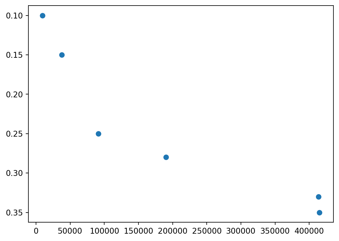
From NumPy
taxes = np.array([
    [9275, .1],
    [37650, .15],
    [91150, .25],
    [190150, .28],
    [413350, .33],
    [415051, .35]
])
df = pd.DataFrame(taxes) # use "df" for dataframes by convention
df # You'll notice this may look a lot nicer| 0 | 1 | |
|---|---|---|
| 0 | 9275.0 | 0.10 |
| 1 | 37650.0 | 0.15 |
| 2 | 91150.0 | 0.25 |
| 3 | 190150.0 | 0.28 |
| 4 | 413350.0 | 0.33 |
| 5 | 415051.0 | 0.35 |
Get a File
- I will use some nuclear data.
- Usually data will come from your research group or experiments.
- Often stored as a CSV.
- A “.csv” file, for “comma separated value”
- We’ll use “Periodic Table of Elements.csv”
- Spaces in maes are annoying; we’ll manage.
- It’s from here
From a URL
- You can use files on your computer, or…
- From a url.
- But the url must be the address of the file
- Not a page that talks about the file.
- Not a page with the same data but presented in a pretty table.
“Raw” Files
- On GitHub (common place to keep files) these are called “raw” files.
- Note - that ends in
.csv
From File
df = pd.read_csv("https://gist.githubusercontent.com/GoodmanSciences/c2dd862cd38f21b0ad36b8f96b4bf1ee/raw/1d92663004489a5b6926e944c1b3d9ec5c40900e/Periodic%2520Table%2520of%2520Elements.csv")
df| AtomicNumber | Element | Symbol | AtomicMass | NumberofNeutrons | NumberofProtons | NumberofElectrons | Period | Group | Phase | ... | FirstIonization | Density | MeltingPoint | BoilingPoint | NumberOfIsotopes | Discoverer | Year | SpecificHeat | NumberofShells | NumberofValence | |
|---|---|---|---|---|---|---|---|---|---|---|---|---|---|---|---|---|---|---|---|---|---|
| 0 | 1 | Hydrogen | H | 1.007 | 0 | 1 | 1 | 1 | 1.0 | gas | ... | 13.5984 | 0.000090 | 14.175 | 20.28 | 3.0 | Cavendish | 1766.0 | 14.304 | 1 | 1.0 |
| 1 | 2 | Helium | He | 4.002 | 2 | 2 | 2 | 1 | 18.0 | gas | ... | 24.5874 | 0.000179 | NaN | 4.22 | 5.0 | Janssen | 1868.0 | 5.193 | 1 | NaN |
| 2 | 3 | Lithium | Li | 6.941 | 4 | 3 | 3 | 2 | 1.0 | solid | ... | 5.3917 | 0.534000 | 453.850 | 1615.00 | 5.0 | Arfvedson | 1817.0 | 3.582 | 2 | 1.0 |
| 3 | 4 | Beryllium | Be | 9.012 | 5 | 4 | 4 | 2 | 2.0 | solid | ... | 9.3227 | 1.850000 | 1560.150 | 2742.00 | 6.0 | Vaulquelin | 1798.0 | 1.825 | 2 | 2.0 |
| 4 | 5 | Boron | B | 10.811 | 6 | 5 | 5 | 2 | 13.0 | solid | ... | 8.2980 | 2.340000 | 2573.150 | 4200.00 | 6.0 | Gay-Lussac | 1808.0 | 1.026 | 2 | 3.0 |
| ... | ... | ... | ... | ... | ... | ... | ... | ... | ... | ... | ... | ... | ... | ... | ... | ... | ... | ... | ... | ... | ... |
| 113 | 114 | Flerovium | Fl | 289.000 | 175 | 114 | 114 | 7 | 14.0 | artificial | ... | NaN | NaN | NaN | NaN | NaN | NaN | 1999.0 | NaN | 7 | 4.0 |
| 114 | 115 | Moscovium | Mc | 288.000 | 173 | 115 | 115 | 7 | 15.0 | artificial | ... | NaN | NaN | NaN | NaN | NaN | NaN | 2010.0 | NaN | 7 | 5.0 |
| 115 | 116 | Livermorium | Lv | 292.000 | 176 | 116 | 116 | 7 | 16.0 | artificial | ... | NaN | NaN | NaN | NaN | NaN | NaN | 2000.0 | NaN | 7 | 6.0 |
| 116 | 117 | Tennessine | Ts | 295.000 | 178 | 117 | 117 | 7 | 17.0 | artificial | ... | NaN | NaN | NaN | NaN | NaN | NaN | 2010.0 | NaN | 7 | 7.0 |
| 117 | 118 | Oganesson | Og | 294.000 | 176 | 118 | 118 | 7 | 18.0 | artificial | ... | NaN | NaN | NaN | NaN | NaN | NaN | 2006.0 | NaN | 7 | 8.0 |
118 rows × 28 columns
DataFrames
DataFrames and Arrays
- DataFrames:
- Have row and column labels
- Can store multiple types of data (strings/words, integers, and floating point numbers)
- Arrays:
- Don’t
- Can’t
Subsetting
- One of the most common uses for pandas is to subset, to look at part of DataFrame but not all.
- Usually by looking at a specific column or columns - by name.
- Vs. arrays and lists, DataFrames still have indices, but they are now usually strings.
Multiple Indices
- We can also subset multiple indices using a list of indices (column names).
Filtering
- We can subset rows by filtering
- Basically we write what would be an
ifstatement, but use it as an index. - The “transuranic” elements are elements higher than number 92.
| AtomicNumber | Element | Symbol | AtomicMass | NumberofNeutrons | NumberofProtons | NumberofElectrons | Period | Group | Phase | ... | FirstIonization | Density | MeltingPoint | BoilingPoint | NumberOfIsotopes | Discoverer | Year | SpecificHeat | NumberofShells | NumberofValence | |
|---|---|---|---|---|---|---|---|---|---|---|---|---|---|---|---|---|---|---|---|---|---|
| 92 | 93 | Neptunium | Np | 237.0 | 144 | 93 | 93 | 7 | NaN | artificial | ... | 6.2657 | 20.5 | 913.15 | 4273.0 | 153.0 | McMillan and Abelson | 1940.0 | NaN | 7 | NaN |
| 93 | 94 | Plutonium | Pu | 244.0 | 150 | 94 | 94 | 7 | NaN | artificial | ... | 6.0262 | 19.8 | 913.15 | 3501.0 | 163.0 | Seaborg et al. | 1940.0 | NaN | 7 | NaN |
| 94 | 95 | Americium | Am | 243.0 | 148 | 95 | 95 | 7 | NaN | artificial | ... | 5.9738 | 13.7 | 1267.15 | 2880.0 | 133.0 | Seaborg et al. | 1944.0 | NaN | 7 | NaN |
| 95 | 96 | Curium | Cm | 247.0 | 151 | 96 | 96 | 7 | NaN | artificial | ... | 5.9915 | 13.5 | 1340.15 | 3383.0 | 133.0 | Seaborg et al. | 1944.0 | NaN | 7 | NaN |
| 96 | 97 | Berkelium | Bk | 247.0 | 150 | 97 | 97 | 7 | NaN | artificial | ... | 6.1979 | 14.8 | 1259.15 | 983.0 | 83.0 | Seaborg et al. | 1949.0 | NaN | 7 | NaN |
| 97 | 98 | Californium | Cf | 251.0 | 153 | 98 | 98 | 7 | NaN | artificial | ... | 6.2817 | 15.1 | 1925.15 | 1173.0 | 123.0 | Seaborg et al. | 1950.0 | NaN | 7 | NaN |
| 98 | 99 | Einsteinium | Es | 252.0 | 153 | 99 | 99 | 7 | NaN | artificial | ... | 6.4200 | 13.5 | 1133.15 | NaN | 123.0 | Ghiorso et al. | 1952.0 | NaN | 7 | NaN |
| 99 | 100 | Fermium | Fm | 257.0 | 157 | 100 | 100 | 7 | NaN | artificial | ... | 6.5000 | NaN | NaN | NaN | 103.0 | Ghiorso et al. | 1953.0 | NaN | 7 | NaN |
| 100 | 101 | Mendelevium | Md | 258.0 | 157 | 101 | 101 | 7 | NaN | artificial | ... | 6.5800 | NaN | NaN | NaN | 33.0 | Ghiorso et al. | 1955.0 | NaN | 7 | NaN |
| 101 | 102 | Nobelium | No | 259.0 | 157 | 102 | 102 | 7 | NaN | artificial | ... | 6.6500 | NaN | NaN | NaN | 73.0 | Ghiorso et al. | 1958.0 | NaN | 7 | NaN |
| 102 | 103 | Lawrencium | Lr | 262.0 | 159 | 103 | 103 | 7 | NaN | artificial | ... | NaN | NaN | NaN | NaN | 203.0 | Ghiorso et al. | 1961.0 | NaN | 7 | NaN |
| 103 | 104 | Rutherfordium | Rf | 261.0 | 157 | 104 | 104 | 7 | 4.0 | artificial | ... | NaN | 18.1 | NaN | NaN | NaN | Ghiorso et al. | 1969.0 | NaN | 7 | NaN |
| 104 | 105 | Dubnium | Db | 262.0 | 157 | 105 | 105 | 7 | 5.0 | artificial | ... | NaN | 39.0 | NaN | NaN | NaN | Ghiorso et al. | 1970.0 | NaN | 7 | NaN |
| 105 | 106 | Seaborgium | Sg | 266.0 | 160 | 106 | 106 | 7 | 6.0 | artificial | ... | NaN | 35.0 | NaN | NaN | NaN | Ghiorso et al. | 1974.0 | NaN | 7 | NaN |
| 106 | 107 | Bohrium | Bh | 264.0 | 157 | 107 | 107 | 7 | 7.0 | artificial | ... | NaN | 37.0 | NaN | NaN | NaN | Armbruster and M�nzenberg | 1981.0 | NaN | 7 | NaN |
| 107 | 108 | Hassium | Hs | 267.0 | 159 | 108 | 108 | 7 | 8.0 | artificial | ... | NaN | 41.0 | NaN | NaN | NaN | Armbruster and M�nzenberg | 1983.0 | NaN | 7 | NaN |
| 108 | 109 | Meitnerium | Mt | 268.0 | 159 | 109 | 109 | 7 | 9.0 | artificial | ... | NaN | 35.0 | NaN | NaN | NaN | GSI, Darmstadt, West Germany | 1982.0 | NaN | 7 | NaN |
| 109 | 110 | Darmstadtium | Ds | 271.0 | 161 | 110 | 110 | 7 | 10.0 | artificial | ... | NaN | NaN | NaN | NaN | NaN | NaN | 1994.0 | NaN | 7 | NaN |
| 110 | 111 | Roentgenium | Rg | 272.0 | 161 | 111 | 111 | 7 | 11.0 | artificial | ... | NaN | NaN | NaN | NaN | NaN | NaN | 1994.0 | NaN | 7 | NaN |
| 111 | 112 | Copernicium | Cn | 285.0 | 173 | 112 | 112 | 7 | 12.0 | artificial | ... | NaN | NaN | NaN | NaN | NaN | NaN | 1996.0 | NaN | 7 | NaN |
| 112 | 113 | Nihonium | Nh | 284.0 | 171 | 113 | 113 | 7 | 13.0 | artificial | ... | NaN | NaN | NaN | NaN | NaN | NaN | 2004.0 | NaN | 7 | 3.0 |
| 113 | 114 | Flerovium | Fl | 289.0 | 175 | 114 | 114 | 7 | 14.0 | artificial | ... | NaN | NaN | NaN | NaN | NaN | NaN | 1999.0 | NaN | 7 | 4.0 |
| 114 | 115 | Moscovium | Mc | 288.0 | 173 | 115 | 115 | 7 | 15.0 | artificial | ... | NaN | NaN | NaN | NaN | NaN | NaN | 2010.0 | NaN | 7 | 5.0 |
| 115 | 116 | Livermorium | Lv | 292.0 | 176 | 116 | 116 | 7 | 16.0 | artificial | ... | NaN | NaN | NaN | NaN | NaN | NaN | 2000.0 | NaN | 7 | 6.0 |
| 116 | 117 | Tennessine | Ts | 295.0 | 178 | 117 | 117 | 7 | 17.0 | artificial | ... | NaN | NaN | NaN | NaN | NaN | NaN | 2010.0 | NaN | 7 | 7.0 |
| 117 | 118 | Oganesson | Og | 294.0 | 176 | 118 | 118 | 7 | 18.0 | artificial | ... | NaN | NaN | NaN | NaN | NaN | NaN | 2006.0 | NaN | 7 | 8.0 |
26 rows × 28 columns
Double df
- We use
dftwice in that expression:- Once to check the
dfif some value is greater than 92 - Once to look up all elements for which the value is greater.
- Once to check the
.columns
- By the way, what all do we know?
Index(['AtomicNumber', 'Element', 'Symbol', 'AtomicMass', 'NumberofNeutrons',
       'NumberofProtons', 'NumberofElectrons', 'Period', 'Group', 'Phase',
       'Radioactive', 'Natural', 'Metal', 'Nonmetal', 'Metalloid', 'Type',
       'AtomicRadius', 'Electronegativity', 'FirstIonization', 'Density',
       'MeltingPoint', 'BoilingPoint', 'NumberOfIsotopes', 'Discoverer',
       'Year', 'SpecificHeat', 'NumberofShells', 'NumberofValence'],
dtype='object')- Oh that’s a lot of information!
How big?
- How big is
df?
- And by the way,
np.array’s haveshapetoo.
- Aside: Multiple values within a
()are asically lists but called tuples.
Locating Entries
- Sometimes you want to use an integer index.
AtomicNumber                   11
Element                    Sodium
Symbol                         Na
AtomicMass                  22.99
NumberofNeutrons               12
NumberofProtons                11
NumberofElectrons              11
Period                          3
Group                         1.0
Phase                       solid
Radioactive                   NaN
Natural                       yes
Metal                         yes
Nonmetal                      NaN
Metalloid                     NaN
Type                 Alkali Metal
AtomicRadius                  2.2
Electronegativity            0.93
FirstIonization            5.1391
Density                     0.971
MeltingPoint               371.15
BoilingPoint               1156.0
NumberOfIsotopes              7.0
Discoverer                   Davy
Year                       1807.0
SpecificHeat                1.228
NumberofShells                  3
NumberofValence               1.0
Name: 10, dtype: object
Zero/One index
- DataFrames are 0-indexed
- Elements are 1-indexed1 with good reason.
Data Manipulation
- Check out these columns
Pattern
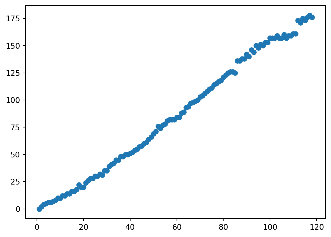
- It looks like atoms with fewer protons have the same number of protons and neutrons, and atoms with many protons have many more neutrons.
- Let’s calculate the difference.
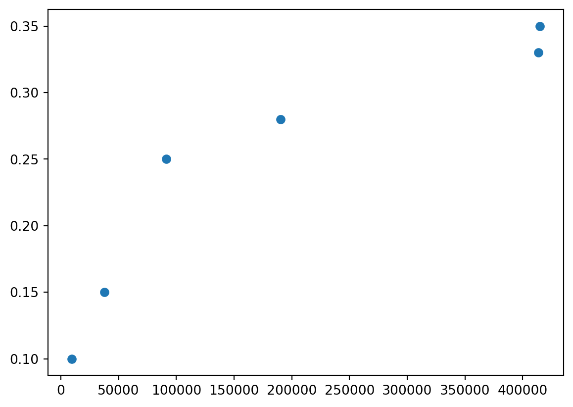
Plots
Visualize
- Easier to visualize.
Scatterplot
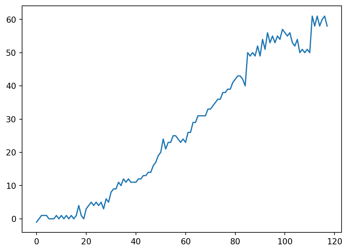
Insights
- A lot of science, as far as I can tell is finding novel insights.
- I noticed that boiling/melting point seemed to go up and down at some intervals.
- I recall that the number of outermost electrons did that too…
- Let’s make
num_esagain, from last time.
num_es
es = np.array([2, 8, 8, 18, 18, 32, 32])
num_es = np.array([]) # The first zero elements
for e in es:
    num_es = np.append(num_es, np.arange(e))
num_es += 1
num_es
array([ 1., 2., 1., 2., 3., 4., 5., 6., 7., 8., 1., 2., 3.,
4., 5., 6., 7., 8., 1., 2., 3., 4., 5., 6., 7., 8.,
9., 10., 11., 12., 13., 14., 15., 16., 17., 18., 1., 2., 3.,
4., 5., 6., 7., 8., 9., 10., 11., 12., 13., 14., 15., 16.,
17., 18., 1., 2., 3., 4., 5., 6., 7., 8., 9., 10., 11.,
12., 13., 14., 15., 16., 17., 18., 19., 20., 21., 22., 23., 24.,
25., 26., 27., 28., 29., 30., 31., 32., 1., 2., 3., 4., 5.,
6., 7., 8., 9., 10., 11., 12., 13., 14., 15., 16., 17., 18.,
19., 20., 21., 22., 23., 24., 25., 26., 27., 28., 29., 30., 31.,
32.])Expanding DataFrames
- We can create a new column and add new data to it from a
np.array - At least if the dimensions work out…
- We have 118 elements, so it is good we have 118 possible outermost electron counts!
Update list
- Like updating the element of a list by index…
Update DataFrame
- We can update or add a column to a DataFrame by index:
Patterns
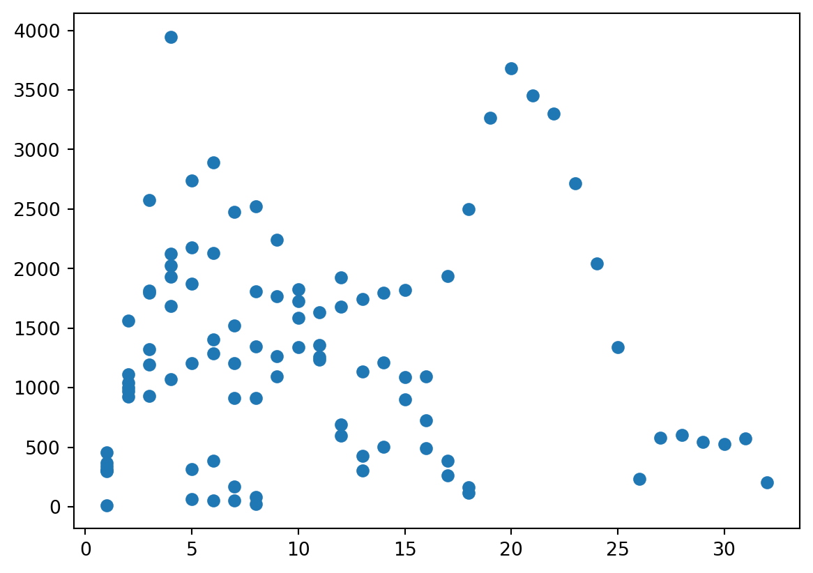
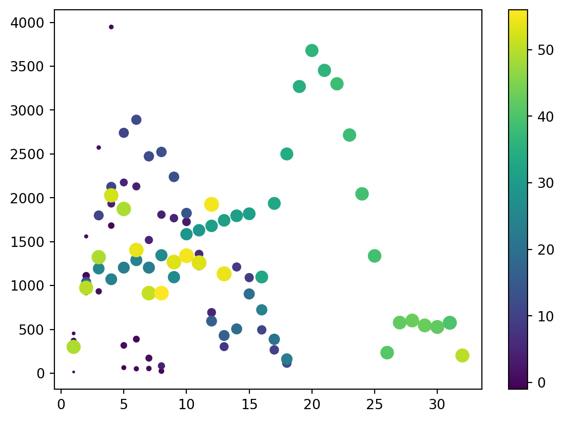
- For a scatter, that is two (
2) DataFrames (or subsets), not one DataFrame with two columns
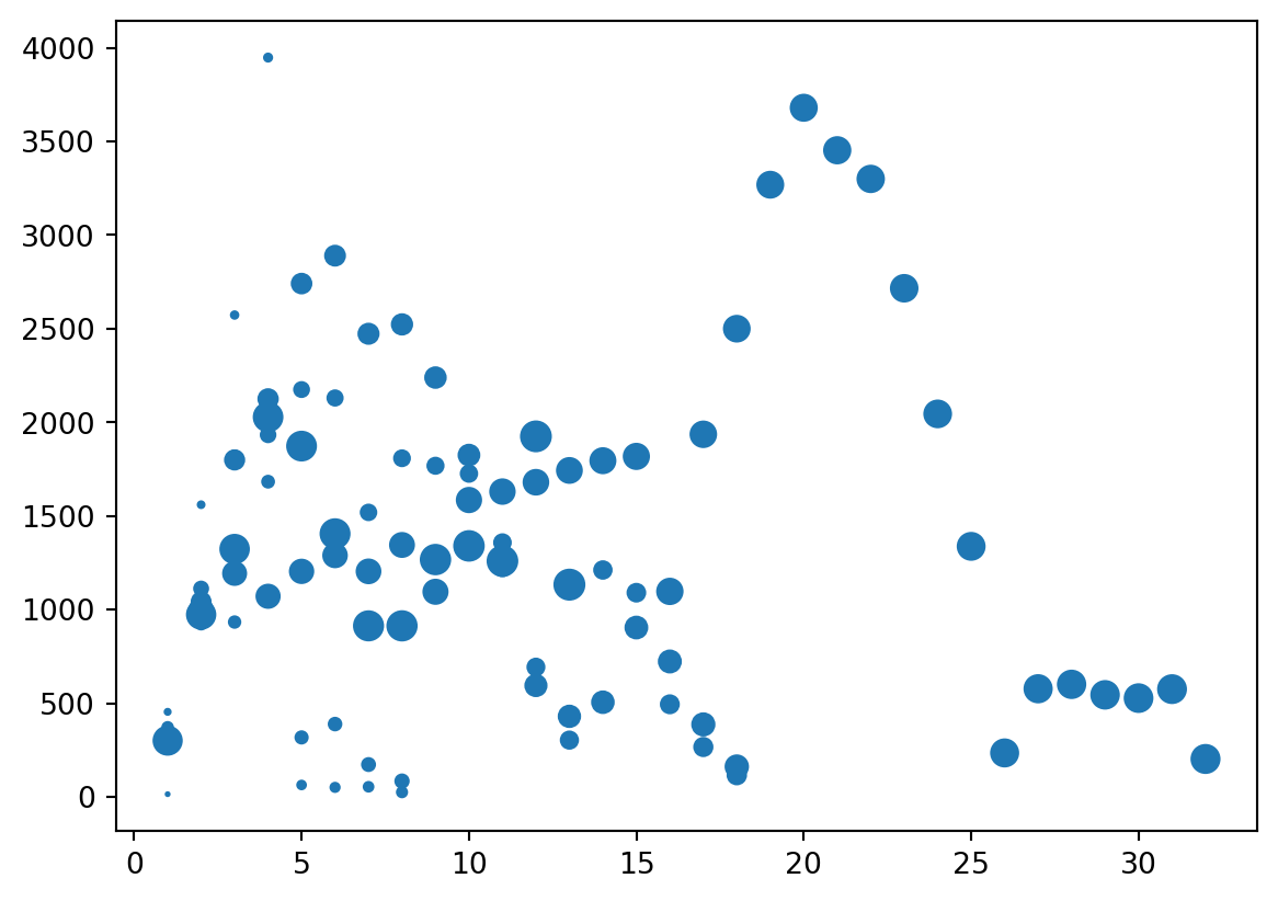
3D
- Third dimension via
s=for size
Columns to Columns
- Using vector operations, we can make novel columns from existing columns.
4D
“kwargs”
- When we call a function and use something like
x=in the arguments,xis a keyword so we call these “kwargs” for “keyword arguments”. - You may see this when looking up functions.
- Just follow examples.
Dropping
- Some columns may be useless or redundant.
Drop it
- We can remove such columns.
Summaries
Summary Statistics
- There’s a variety of ways to describe a DataFrame other than just seeing all of it’s data.
| AtomicNumber | AtomicMass | NumberofNeutrons | Period | Group | AtomicRadius | Electronegativity | FirstIonization | Density | MeltingPoint | BoilingPoint | NumberOfIsotopes | Year | SpecificHeat | NumberofShells | NumberofValence | OutermostElectrons | NeutronsLessProtons | |
|---|---|---|---|---|---|---|---|---|---|---|---|---|---|---|---|---|---|---|
| count | 118.000000 | 118.000000 | 118.000000 | 118.000000 | 90.000000 | 86.000000 | 96.000000 | 102.000000 | 105.000000 | 98.000000 | 98.000000 | 103.000000 | 107.000000 | 85.000000 | 118.000000 | 49.000000 | 118.000000 | 118.000000 |
| mean | 59.500000 | 145.988297 | 86.483051 | 5.254237 | 9.944444 | 1.825814 | 1.695000 | 7.988505 | 9.232161 | 1281.475184 | 2513.143163 | 28.116505 | 1865.280374 | 0.635976 | 5.254237 | 4.428571 | 12.483051 | 26.983051 |
| std | 34.207699 | 88.954899 | 54.785320 | 1.618200 | 5.597674 | 0.611058 | 0.621174 | 3.334571 | 8.630406 | 903.685175 | 1601.901036 | 35.864205 | 97.951740 | 1.653965 | 1.618200 | 2.345208 | 8.830535 | 20.782547 |
| min | 1.000000 | 1.007000 | 0.000000 | 1.000000 | 1.000000 | 0.490000 | 0.700000 | 3.893900 | 0.000090 | 14.175000 | 4.220000 | 3.000000 | 1250.000000 | 0.094000 | 1.000000 | 1.000000 | 1.000000 | -1.000000 |
| 25% | 30.250000 | 66.465750 | 36.000000 | 4.000000 | 5.000000 | 1.425000 | 1.237500 | 6.004850 | 2.700000 | 510.695000 | 1069.000000 | 11.000000 | 1803.500000 | 0.168000 | 4.000000 | 2.000000 | 5.000000 | 6.500000 |
| 50% | 59.500000 | 142.575000 | 83.000000 | 6.000000 | 10.500000 | 1.800000 | 1.585000 | 6.960250 | 7.290000 | 1204.150000 | 2767.000000 | 19.000000 | 1878.000000 | 0.244000 | 6.000000 | 4.000000 | 11.000000 | 24.500000 |
| 75% | 88.750000 | 226.750000 | 138.000000 | 7.000000 | 15.000000 | 2.200000 | 2.062500 | 8.964925 | 12.000000 | 1811.150000 | 3596.750000 | 24.000000 | 1940.000000 | 0.489000 | 7.000000 | 6.000000 | 18.000000 | 49.750000 |
| max | 118.000000 | 295.000000 | 178.000000 | 7.000000 | 18.000000 | 3.300000 | 3.980000 | 24.587400 | 41.000000 | 3948.150000 | 5869.000000 | 203.000000 | 2010.000000 | 14.304000 | 7.000000 | 8.000000 | 32.000000 | 61.000000 |
Info
- Info is often helpful
<class 'pandas.core.frame.DataFrame'>
RangeIndex: 118 entries, 0 to 117
Data columns (total 28 columns):
 #   Column               Non-Null Count  Dtype
---  ------               --------------  -----
 0   AtomicNumber         118 non-null    int64
 1   Element              118 non-null    object
 2   Symbol               118 non-null    object
 3   AtomicMass           118 non-null    float64
 4   NumberofNeutrons     118 non-null    int64
 5   Period               118 non-null    int64
 6   Group                90 non-null     float64
 7   Phase                118 non-null    object
 8   Radioactive          37 non-null     object
 9   Natural              90 non-null     object
 10  Metal                92 non-null     object
 11  Nonmetal             19 non-null     object
 12  Metalloid            7 non-null      object
 13  Type                 115 non-null    object
 14  AtomicRadius         86 non-null     float64
 15  Electronegativity    96 non-null     float64
 16  FirstIonization      102 non-null    float64
 17  Density              105 non-null    float64
 18  MeltingPoint         98 non-null     float64
 19  BoilingPoint         98 non-null     float64
 20  NumberOfIsotopes     103 non-null    float64
 21  Discoverer           109 non-null    object
 22  Year                 107 non-null    float64
 23  SpecificHeat         85 non-null     float64
 24  NumberofShells       118 non-null    int64
 25  NumberofValence      49 non-null     float64
 26  OutermostElectrons   118 non-null    float64
 27  NeutronsLessProtons  118 non-null    int64
dtypes: float64(13), int64(5), object(10)
memory usage: 25.9+ KB
Columns
- And remember we can see all the column names!
- No
()!
Index(['AtomicNumber', 'Element', 'Symbol', 'AtomicMass', 'NumberofNeutrons',
       'Period', 'Group', 'Phase', 'Radioactive', 'Natural', 'Metal',
       'Nonmetal', 'Metalloid', 'Type', 'AtomicRadius', 'Electronegativity',
       'FirstIonization', 'Density', 'MeltingPoint', 'BoilingPoint',
       'NumberOfIsotopes', 'Discoverer', 'Year', 'SpecificHeat',
       'NumberofShells', 'NumberofValence', 'OutermostElectrons',
       'NeutronsLessProtons'],
      dtype='object')
Shape
- And of course shape!
Column-wise
- We can do all kinds of operations over a single column.
mp = df["MeltingPoint"] # Copy column to save some typing.
[mp.min(), mp.max(), mp.mean(), mp.median(), mp.mode(), mp.std()]
[np.float64(14.175),
np.float64(3948.15),
np.float64(1281.4751836734692),
np.float64(1204.15),
0 913.15
1 1204.15
Name: MeltingPoint, dtype: float64,
np.float64(903.6851752147392)]Using loc
Metal or not
- We helpfully can already see what metals are.
NaN
NaNmeans “not a number” and is used by pandas (not generally by Python) to fill in missing data.
C:\Users\cd-desk\AppData\Local\Temp\ipykernel_12296\3438155168.py:1: RuntimeWarning:

invalid value encountered in sqrt
np.float64(nan)- I find this idea a bit odd (and e.g. Polars does not do this) but we can work with it.
(Non)metal(loid)
- Elements are “metal”, “nonmetal”, or “metalloid”.
- I regard this as how metallic an element is.
Metallic
- We introduce and use
np.where, which takes- A condition
- A value if condition
- A value else
Metalloids
- Additionally deal with metalloids.
df[df["Metalloid"] == "yes"]["Metallic"] = "Metalloid"
df.iloc[12:16][["Metal","Nonmetal","Metalloid","Metallic"]]
C:\Users\cd-desk\AppData\Local\Temp\ipykernel_12296\1792942652.py:1: SettingWithCopyWarning:
A value is trying to be set on a copy of a slice from a DataFrame.
Try using .loc[row_indexer,col_indexer] = value instead
See the caveats in the documentation: https://pandas.pydata.org/pandas-docs/stable/user_guide/indexing.html#returning-a-view-versus-a-copy
| Metal | Nonmetal | Metalloid | Metallic | |
|---|---|---|---|---|
| 12 | yes | NaN | NaN | Metal |
| 13 | NaN | NaN | yes | Nonmetal |
| 14 | NaN | yes | NaN | Nonmetal |
| 15 | NaN | yes | NaN | Nonmetal |
- Whoops!
loc
df[df["Metalloid"] == "yes"]is not the same dataframe asdf- Changes to it will not change
df. - We use
.loc, the cousin of.ilocto updatedf. - We must also very carefully put all indices, comma separated, in single brackets.
- Row and column, together, within
[]
- Row and column, together, within
Recall: NumPy
- I recommend using the comma notation.
- Otherwise I get unexpected behavior.
- Takeaway: Always use
[x,y]instead of[x][y] - This is why we use
NumPypandas!
Update
df.loc[df["Metalloid"] == "yes", "Metallic"] = "Metalloid"
df.iloc[12:16][["Metal","Nonmetal","Metalloid","Metallic"]]| Metal | Nonmetal | Metalloid | Metallic | |
|---|---|---|---|---|
| 12 | yes | NaN | NaN | Metal |
| 13 | NaN | NaN | yes | Metalloid |
| 14 | NaN | yes | NaN | Nonmetal |
| 15 | NaN | yes | NaN | Nonmetal |
- Much nicer.
Another drop
- Let’s just keep “Metallic” now that we have it.
# Have to specify columns (we can also drop rows)
df = df.drop(columns=["Metal","Nonmetal","Metalloid"])
df.columns
Index(['AtomicNumber', 'Element', 'Symbol', 'AtomicMass', 'NumberofNeutrons',
'Period', 'Group', 'Phase', 'Radioactive', 'Natural', 'Type',
'AtomicRadius', 'Electronegativity', 'FirstIonization', 'Density',
'MeltingPoint', 'BoilingPoint', 'NumberOfIsotopes', 'Discoverer',
'Year', 'SpecificHeat', 'NumberofShells', 'NumberofValence',
'OutermostElectrons', 'NeutronsLessProtons', 'Metallic'],
dtype='object')Groups
On groups
- In chemistry:
a group (also known as a family) is a column of elements in the periodic table of the chemical elements.
- In computing
a set together with a binary operation satisfying certain algebraic conditions.
On groupby
- In pandas
A
groupbyoperation involves some combination of splitting the object, applying a function, and combining the results. This can be used to group large amounts of data and compute operations on these groups.
Element Groups
Counting
- Let’s see how many elements are in each group!
| AtomicNumber | Element | Symbol | AtomicMass | NumberofNeutrons | Period | Phase | Radioactive | Natural | Type | ... | BoilingPoint | NumberOfIsotopes | Discoverer | Year | SpecificHeat | NumberofShells | NumberofValence | OutermostElectrons | NeutronsLessProtons | Metallic | |
|---|---|---|---|---|---|---|---|---|---|---|---|---|---|---|---|---|---|---|---|---|---|
| Group | |||||||||||||||||||||
| 1.0 | 7 | 7 | 7 | 7 | 7 | 7 | 7 | 1 | 7 | 7 | ... | 7 | 7 | 7 | 7 | 6 | 7 | 7 | 7 | 7 | 7 |
| 2.0 | 6 | 6 | 6 | 6 | 6 | 6 | 6 | 1 | 6 | 6 | ... | 6 | 6 | 6 | 6 | 5 | 6 | 6 | 6 | 6 | 6 |
| 3.0 | 4 | 4 | 4 | 4 | 4 | 4 | 4 | 1 | 4 | 4 | ... | 4 | 4 | 4 | 4 | 4 | 4 | 0 | 4 | 4 | 4 |
| 4.0 | 4 | 4 | 4 | 4 | 4 | 4 | 4 | 1 | 3 | 4 | ... | 3 | 3 | 4 | 4 | 3 | 4 | 0 | 4 | 4 | 4 |
| 5.0 | 4 | 4 | 4 | 4 | 4 | 4 | 4 | 1 | 3 | 4 | ... | 3 | 3 | 4 | 4 | 3 | 4 | 0 | 4 | 4 | 4 |
| 6.0 | 4 | 4 | 4 | 4 | 4 | 4 | 4 | 1 | 3 | 4 | ... | 3 | 3 | 4 | 4 | 3 | 4 | 0 | 4 | 4 | 4 |
| 7.0 | 4 | 4 | 4 | 4 | 4 | 4 | 4 | 2 | 2 | 4 | ... | 3 | 3 | 4 | 4 | 2 | 4 | 0 | 4 | 4 | 4 |
| 8.0 | 4 | 4 | 4 | 4 | 4 | 4 | 4 | 1 | 3 | 4 | ... | 3 | 3 | 4 | 3 | 3 | 4 | 0 | 4 | 4 | 4 |
| 9.0 | 4 | 4 | 4 | 4 | 4 | 4 | 4 | 1 | 3 | 4 | ... | 3 | 3 | 4 | 4 | 3 | 4 | 0 | 4 | 4 | 4 |
| 10.0 | 4 | 4 | 4 | 4 | 4 | 4 | 4 | 1 | 3 | 4 | ... | 3 | 3 | 3 | 4 | 3 | 4 | 0 | 4 | 4 | 4 |
| 11.0 | 4 | 4 | 4 | 4 | 4 | 4 | 4 | 1 | 3 | 4 | ... | 3 | 3 | 3 | 1 | 3 | 4 | 0 | 4 | 4 | 4 |
| 12.0 | 4 | 4 | 4 | 4 | 4 | 4 | 4 | 1 | 3 | 4 | ... | 3 | 3 | 3 | 2 | 3 | 4 | 0 | 4 | 4 | 4 |
| 13.0 | 6 | 6 | 6 | 6 | 6 | 6 | 6 | 1 | 5 | 5 | ... | 5 | 5 | 5 | 6 | 5 | 6 | 6 | 6 | 6 | 6 |
| 14.0 | 6 | 6 | 6 | 6 | 6 | 6 | 6 | 1 | 5 | 6 | ... | 5 | 5 | 5 | 3 | 5 | 6 | 6 | 6 | 6 | 6 |
| 15.0 | 6 | 6 | 6 | 6 | 6 | 6 | 6 | 1 | 5 | 5 | ... | 5 | 5 | 5 | 5 | 5 | 6 | 6 | 6 | 6 | 6 |
| 16.0 | 6 | 6 | 6 | 6 | 6 | 6 | 6 | 2 | 5 | 6 | ... | 5 | 5 | 5 | 5 | 4 | 6 | 6 | 6 | 6 | 6 |
| 17.0 | 6 | 6 | 6 | 6 | 6 | 6 | 6 | 2 | 5 | 5 | ... | 5 | 5 | 5 | 6 | 4 | 6 | 6 | 6 | 6 | 6 |
| 18.0 | 7 | 7 | 7 | 7 | 7 | 7 | 7 | 2 | 6 | 7 | ... | 6 | 6 | 6 | 7 | 6 | 7 | 6 | 7 | 7 | 7 |
18 rows × 25 columns
Goofy
- Oh it took the count of all columns.
- But… that isn’t useless?
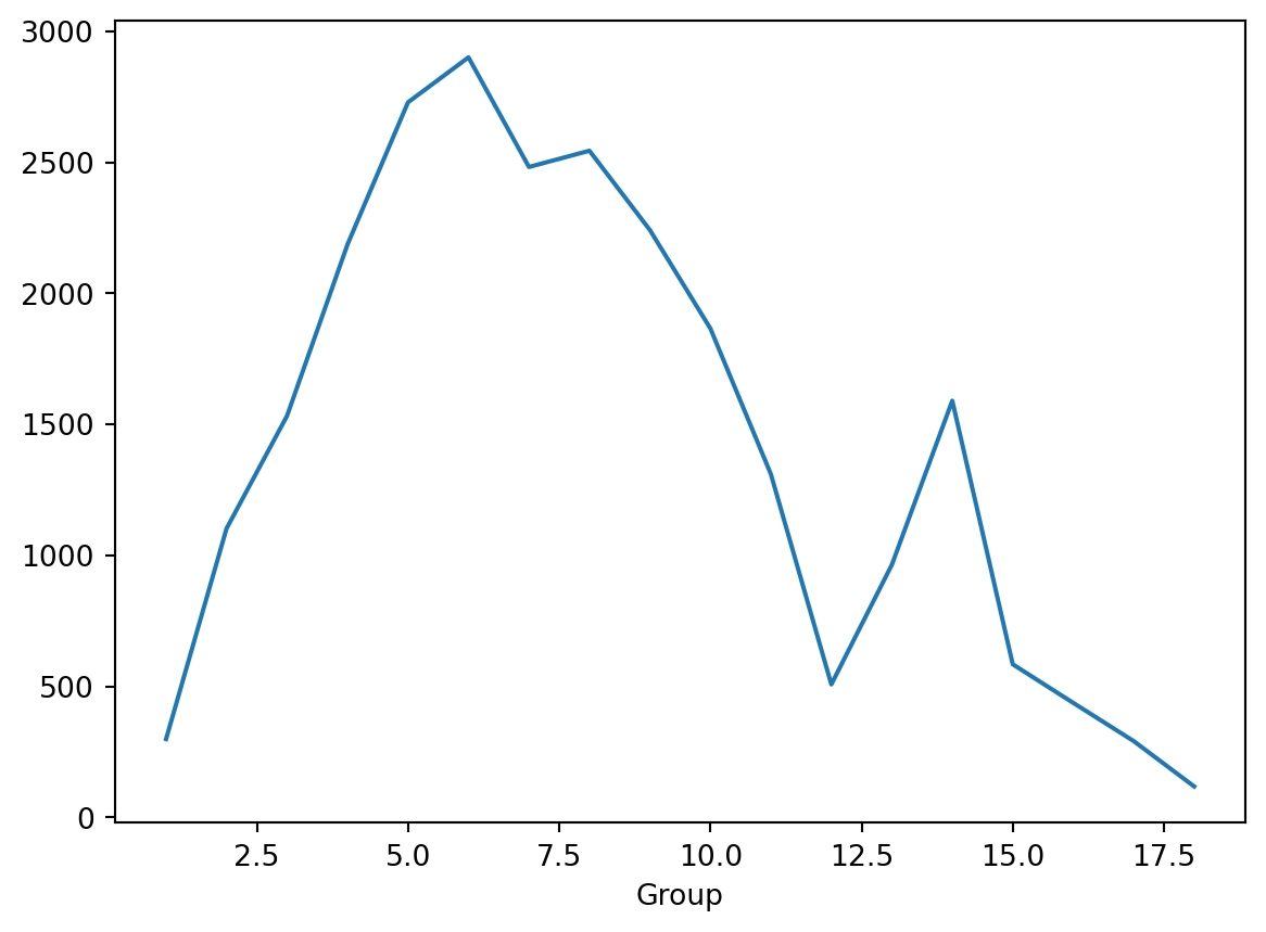
- Let’s perhaps look a melting point by group.
Group
1.0 298.616429
2.0 1102.150000
3.0 1531.900000
4.0 2186.150000
5.0 2728.483333
6.0 2900.150000
7.0 2481.816667
8.0 2543.816667
9.0 2241.150000
10.0 1865.483333
11.0 1309.876667
12.0 507.213333
13.0 963.304000
14.0 1589.742000
15.0 583.882000
16.0 436.622000
17.0 290.758000
18.0 117.638600
Name: MeltingPoint, dtype: float64Plot it
- That was too hard to see.
groupby
- Groupby is a cool and powerful tool.
- I tend to use it with summary statistics, and you can usually work around it with filters, but with a bit of practice it’s a real joy to work with.
Merge
Names
- An astute learning will note a few oddities with names and symbols in the table.
- Some symbols and elements start with different letters.
Strings
- Like lists, arrays, and DataFrames, we can use indices on strings of characters.
Differing
- Sometimes the first letter differs - but not often.
Write a function
- We make a function that checks if two things start with the same letter.
Vectorize
- To apply to DataFrames, we must vectorize it.
x[0]of a DataFrame is a rowx[0]of a string is a letter- We wanted letters!
The Elements
10 Sodium
18 Potassium
25 Iron
46 Silver
49 Tin
50 Antimony
78 Gold
79 Mercury
81 Lead
Name: Element, dtype: object- Basically, these elements have archaic Latin names that were in use when symbols were set before developing their modern names, or something. Read more

Adding Names
- Let’s make another DataFrame
- We’ll call if
adfor “artus datus”, which might (I have no idea) be Latin for data frame.
- We’ll call if
To DataFrame
adfor “artus datus”, which may be Latin for data frame.
Column Names
- Remember
.columns?
Index(['AtomicNumber', 'Element', 'Symbol', 'AtomicMass', 'NumberofNeutrons',
       'Period', 'Group', 'Phase', 'Radioactive', 'Natural', 'Type',
       'AtomicRadius', 'Electronegativity', 'FirstIonization', 'Density',
       'MeltingPoint', 'BoilingPoint', 'NumberOfIsotopes', 'Discoverer',
       'Year', 'SpecificHeat', 'NumberofShells', 'NumberofValence',
       'OutermostElectrons', 'NeutronsLessProtons', 'Metallic'],
dtype='object')- We can actually use
=with.columns
Merge
| AtomicNumber | Element | Symbol | AtomicMass | NumberofNeutrons | Period | Group | Phase | Radioactive | Natural | ... | NumberOfIsotopes | Discoverer | Year | SpecificHeat | NumberofShells | NumberofValence | OutermostElectrons | NeutronsLessProtons | Metallic | Latin | |
|---|---|---|---|---|---|---|---|---|---|---|---|---|---|---|---|---|---|---|---|---|---|
| 0 | 11 | Sodium | Na | 22.990 | 12 | 3 | 1.0 | solid | NaN | yes | ... | 7.0 | Davy | 1807.0 | 1.228 | 3 | 1.0 | 1.0 | 1 | Metal | Natrium |
| 1 | 19 | Potassium | K | 39.098 | 20 | 4 | 1.0 | solid | NaN | yes | ... | 10.0 | Davy | 1807.0 | 0.757 | 4 | 1.0 | 1.0 | 1 | Metal | Kalium |
| 2 | 26 | Iron | Fe | 55.845 | 30 | 4 | 8.0 | solid | NaN | yes | ... | 10.0 | Prehistoric | NaN | 0.449 | 4 | NaN | 8.0 | 4 | Metal | Ferrum |
| 3 | 47 | Silver | Ag | 107.868 | 61 | 5 | 11.0 | solid | NaN | yes | ... | 27.0 | Prehistoric | NaN | 0.235 | 5 | NaN | 11.0 | 14 | Metal | Argentum |
| 4 | 50 | Tin | Sn | 118.710 | 69 | 5 | 14.0 | solid | NaN | yes | ... | 28.0 | Prehistoric | NaN | 0.228 | 5 | 4.0 | 14.0 | 19 | Metal | Stannum |
| 5 | 51 | Antimony | Sb | 121.760 | 71 | 5 | 15.0 | solid | NaN | yes | ... | 29.0 | Early historic times | NaN | 0.207 | 5 | 5.0 | 15.0 | 20 | Metalloid | Stibium |
| 6 | 79 | Gold | Au | 196.967 | 118 | 6 | 11.0 | solid | NaN | yes | ... | 21.0 | Prehistoric | NaN | 0.129 | 6 | NaN | 25.0 | 39 | Metal | Aurum |
| 7 | 80 | Mercury | Hg | 200.590 | 121 | 6 | 12.0 | liq | NaN | yes | ... | 26.0 | Prehistoric | NaN | 0.140 | 6 | NaN | 26.0 | 41 | Metal | Hydrargyrum |
| 8 | 82 | Lead | Pb | 207.200 | 125 | 6 | 14.0 | solid | NaN | yes | ... | 29.0 | Prehistoric | NaN | 0.129 | 6 | 4.0 | 28.0 | 43 | Metal | Plumbum |
9 rows × 27 columns
Oh no!
- So we successfully added Latin names, but…
- We lost all elements without a Latin name.
- The merge only kept elements in both
dfandad
Join
Don’t merge
- In my experience, merges never work, but…
- They explain how joins, the good thing, work.
Background
- To make learning joins easier, we’ll work with two DataFrames.
Index
- Versus
merge, which just figures it out,joinlikes to look at indices. - So we have to make sure we have the same index on both data frames.
- We’ll use
"Symbol"
Simplify
- To make things easier on us, let’s just only look at a few columns.
- We will avoid having two columns of the same name.
- This is manageable, but let’s learn joins first.
The df’s
Visuals
- I will also visualize this using venn diagrams.
- To my knowledge, there is no graceful way to visualize venn diagrams, but
matplotlib-vennis okay. - I’m spoiler-marking code that shows how I make the venn diagrams.
Code
from matplotlib_venn import venn2, venn2_circles
def show_join(how, left, right, mid):
v = venn2((2, 2, 1), ('metalloids', 'latin_name'))
v.get_patch_by_id('100').set_color('darkblue' if left else 'white')
v.get_patch_by_id('010').set_color('darkblue' if right else 'white')
v.get_patch_by_id('110').set_color('darkblue' if mid else 'white')
v.get_patch_by_id('100').set_alpha(1.0)
v.get_patch_by_id('010').set_alpha(1.0)
v.get_patch_by_id('110').set_alpha(1.0)
venn2_circles((2, 2, 1))
for idx, subset in enumerate(v.subset_labels):
v.subset_labels[idx].set_visible(False)
plt.title("metalloids.join(latin_name, how=\"" + how + "\")")
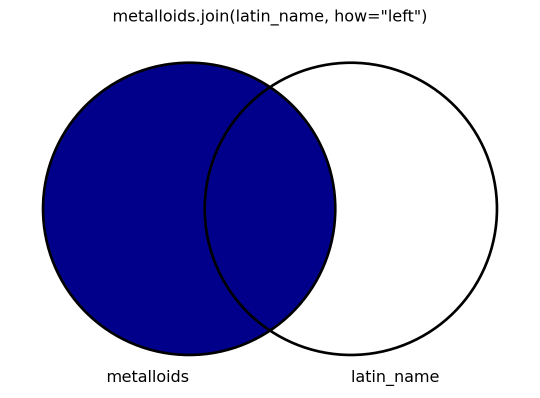
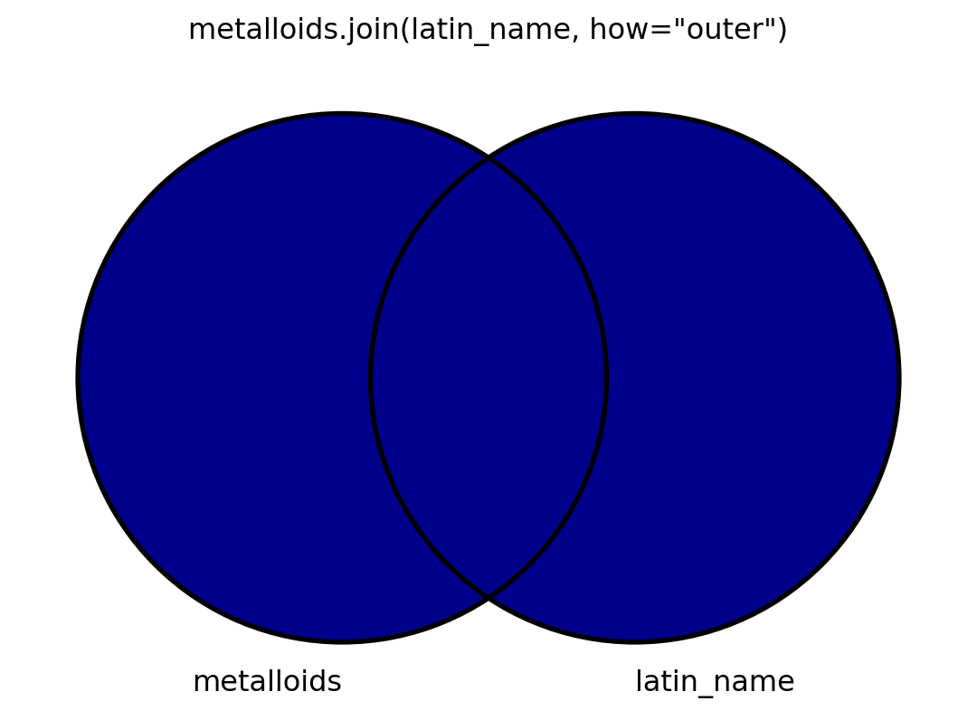
plt.show()Quoth pandas
how: {‘left’,‘right’,‘outer’,‘inner’,‘cross’}
How to handle operation of the two objects.
'left': use calling frame’s index
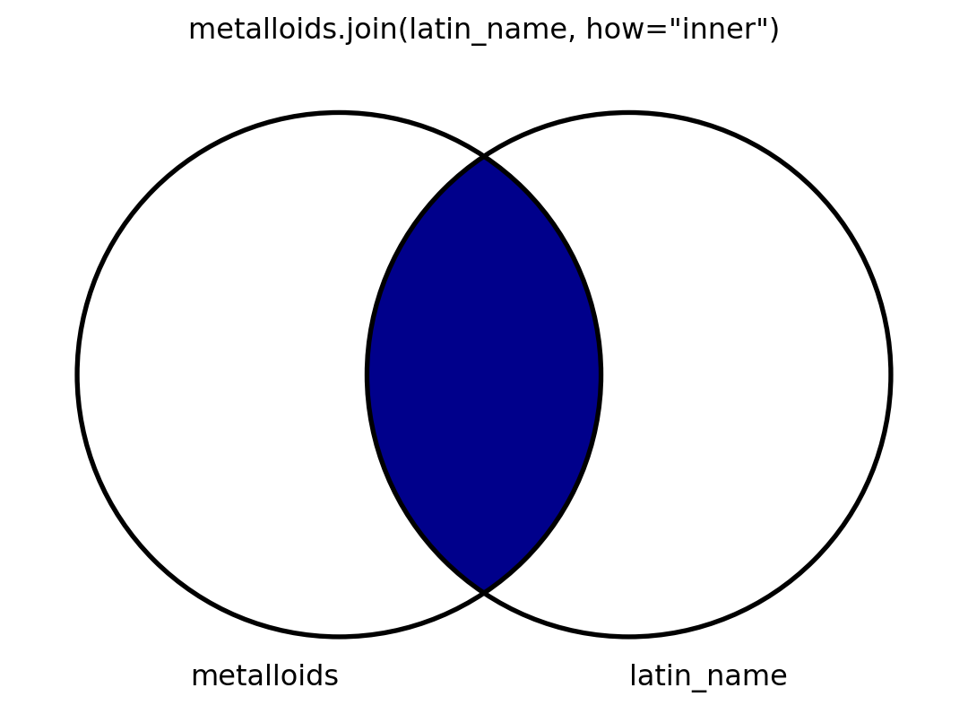
'right': use other’s index.'outer': form union of calling frame’s index with other’s index.'inner': form intersection of calling frame’s index with other’s index.'cross': creates the cartesian product from both frames.
Join
- Join uses all columns, filling with “NaN”.
Left
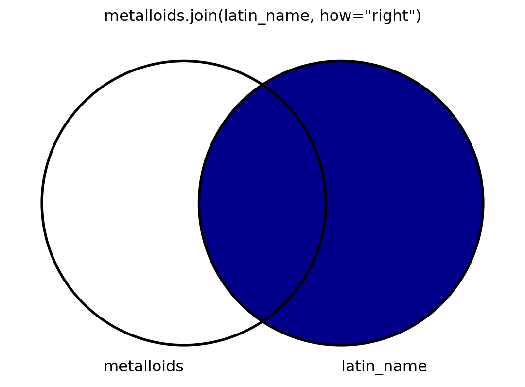
Right
Outer
Inner
Cross
- Cross makes pairs.
- I don’t see it used often.
| AtomicNumber | Metallic | Element | Latin | |
|---|---|---|---|---|
| 0 | 5 | Metalloid | Sodium | Natrium |
| 1 | 5 | Metalloid | Potassium | Kalium |
| 2 | 5 | Metalloid | Iron | Ferrum |
| 3 | 5 | Metalloid | Silver | Argentum |
| 4 | 5 | Metalloid | Tin | Stannum |
| ... | ... | ... | ... | ... |
| 58 | 84 | Metalloid | Tin | Stannum |
| 59 | 84 | Metalloid | Antimony | Stibium |
| 60 | 84 | Metalloid | Gold | Aurum |
| 61 | 84 | Metalloid | Mercury | Hydrargyrum |
| 62 | 84 | Metalloid | Lead | Plumbum |
63 rows × 4 columns
Exercise
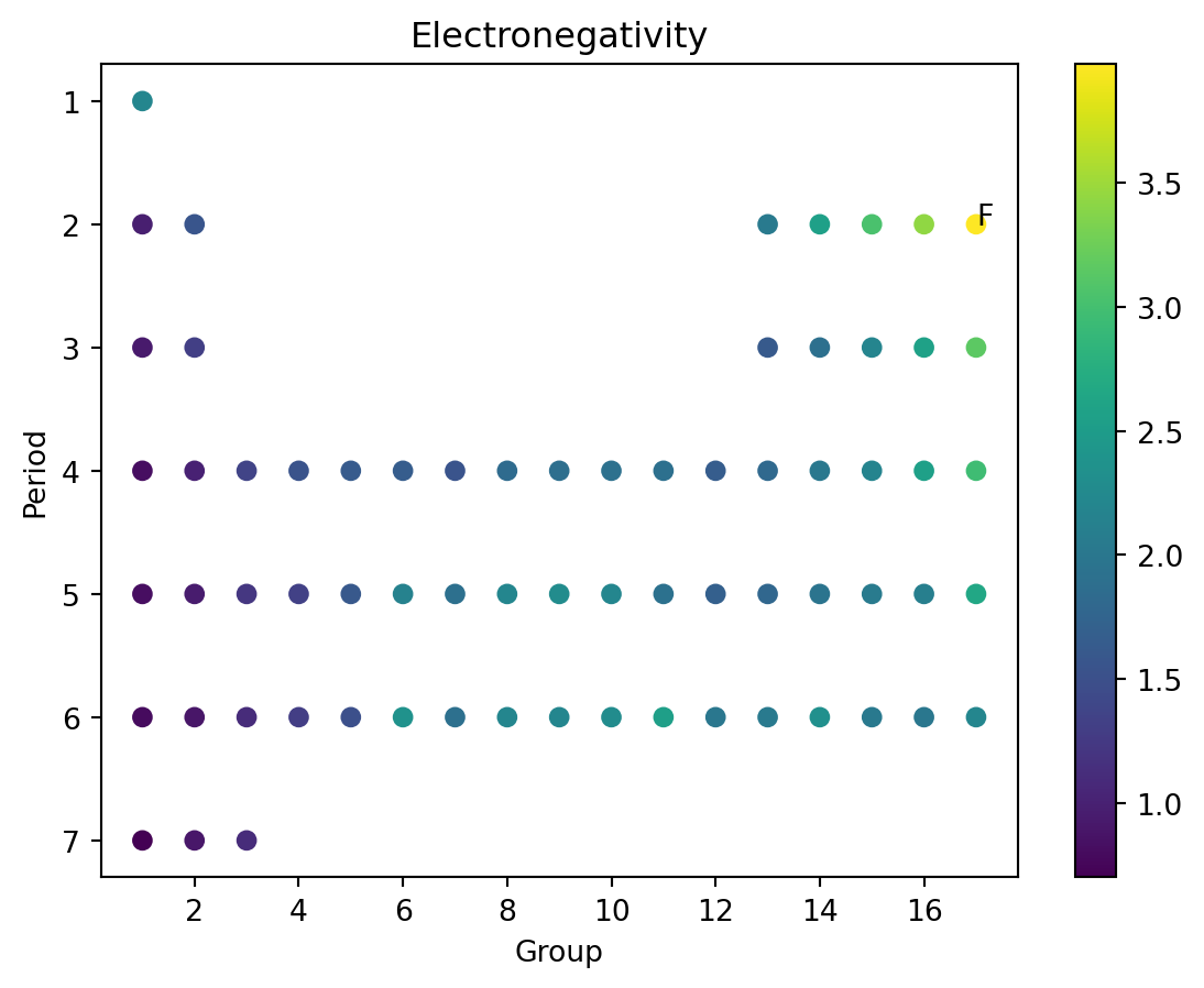
The Table
- The periodic table was developed by laying out elements by “Groups” and “Periods”
- Basically, number of outer electrons (that can bond) and number of layers of inner “shells” of electrons that can’t bond.
- Or something. I’m not a real scientist.
- We can plot these against each other.
Electronegativity
Exercise
- Plot the table, by plotting “Groups” vs “Periods”
- Plot electronegativity using color.
- Confirm the claims from the chemistry text about electronegativity trends.
- Annotate the location of fluorine (F).
Aside: Inversion
- There’s a few ways to invert an axis that you may want to use.
Supply a -
- You can negate, but it impacts labels.
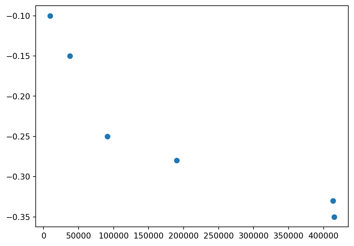
Get axes
- You can use
.gca()(get current axes) and set one negative.
Solution
Footnotes
Neutronium is a proposed but not academically interesting element with atomic number
0.↩︎