Sklearn

Scientific Computing

Why Sklearn?

What is Sklearn?

• Sklearn or scikit-learn, originally conceived as an extension to SciPy.

Scikit-learn is an open source machine learning library that supports supervised and unsupervised learning. It also provides various tools for model fitting, data preprocessing, model selection, model evaluation, and many other utilities.Scikit-learn is an open source machine learning library that supports supervised and unsupervised learning. It also provides various tools for model fitting, data preprocessing, model selection, model evaluation, and many other utilities.

Why sklearn?

• “Simple and efficient tools for predictive data analysis”
• “Accessible to everybody, and reusable in various contexts”
• “Built on NumPy, SciPy, and matplotlib”
• “Open source, commercially usable - BSD license”

Why not sklearn?

• The closest thing to competitors, to my knowledge, are Torch and Tensorflow.
  • The Meta and Google GPU-accelerated frameworks, respectively.
• I don’t like that the other frameworks are managed by big tech companies, and I don’t think they are as well suited to science.

Using Sklearn

• Sklearn/scikit-learn is incrementally more involved to install via pip because, well, sometimes it is called “sklearn” and sometimes “scikit-learn”.
• This gets me almost every time:

$ python3 -m pip install sklearn
Collecting sklearn
  Downloading sklearn-0.0.post12.tar.gz (2.6 kB)
  Preparing metadata (setup.py) ... error
  error: subprocess-exited-with-error

  × python setup.py egg_info did not run successfully.
  │ exit code: 1
  ╰─> [15 lines of output]
      The 'sklearn' PyPI package is deprecated, use 'scikit-learn'
      rather than 'sklearn' for pip commands.

Use scikit-learn

• Scikit-learn recommends the following:

python3 -m pip install scikit-learn
python3 -m pip show scikit-learn  # show scikit-learn version and location
python3 -m pip freeze             # show all installed packages in the environment
python3 -c "import sklearn; sklearn.show_versions()"

• You will see a lot of text.

Easier

• Just open python/python3 and

import sklearn

• Like SciPy, usually parts of Sklearn are imported, so that isn’t an expected two-letter name like np or pd
• I never use sklearn without at least pandas, NumPy, and Matplotlib.

import numpy as np
import pandas as pd
import matplotlib.pyplot as plt

These Slides

• We will focus on cognitive and vision science, motivated by the legendary example that drove early machine learning research…

THE MNIST DATABASE

of handwritten digits

Citation

mnist.bib

@article{lecun1998mnist,
  title={The MNIST database of handwritten digits},
  author={LeCun, Yann},
  journal={http://yann. lecun. com/exdb/mnist/},
  year={1998}
}

Credit

• I will follow this guide:
• Recognizing hand-written digits

The Data

• The MNIST dataset is pretty easy to find, even if the original source isn’t maintained anymore.
• In fairness, it was posted before I started kindergarten
  • German for “children garden”
• It is so much everywhere, it is built into sklearn!

from sklearn import datasets

digits = datasets.load_digits()

Look at it

digits

{'data': array([[ 0.,  0.,  5., ...,  0.,  0.,  0.],
        [ 0.,  0.,  0., ..., 10.,  0.,  0.],
        [ 0.,  0.,  0., ..., 16.,  9.,  0.],
        ...,
        [ 0.,  0.,  1., ...,  6.,  0.,  0.],
        [ 0.,  0.,  2., ..., 12.,  0.,  0.],
        [ 0.,  0., 10., ..., 12.,  1.,  0.]]),
 'target': array([0, 1, 2, ..., 8, 9, 8]),
 'frame': None,
 'feature_names': ['pixel_0_0',
  'pixel_0_1',
  'pixel_0_2',
  'pixel_0_3',
  'pixel_0_4',
  'pixel_0_5',
  'pixel_0_6',
  'pixel_0_7',
  'pixel_1_0',
  'pixel_1_1',
  'pixel_1_2',
  'pixel_1_3',
  'pixel_1_4',
  'pixel_1_5',
  'pixel_1_6',
  'pixel_1_7',
  'pixel_2_0',
  'pixel_2_1',
  'pixel_2_2',
  'pixel_2_3',
  'pixel_2_4',
  'pixel_2_5',
  'pixel_2_6',
  'pixel_2_7',
  'pixel_3_0',
  'pixel_3_1',
  'pixel_3_2',
  'pixel_3_3',
  'pixel_3_4',
  'pixel_3_5',
  'pixel_3_6',
  'pixel_3_7',
  'pixel_4_0',
  'pixel_4_1',
  'pixel_4_2',
  'pixel_4_3',
  'pixel_4_4',
  'pixel_4_5',
  'pixel_4_6',
  'pixel_4_7',
  'pixel_5_0',
  'pixel_5_1',
  'pixel_5_2',
  'pixel_5_3',
  'pixel_5_4',
  'pixel_5_5',
  'pixel_5_6',
  'pixel_5_7',
  'pixel_6_0',
  'pixel_6_1',
  'pixel_6_2',
  'pixel_6_3',
  'pixel_6_4',
  'pixel_6_5',
  'pixel_6_6',
  'pixel_6_7',
  'pixel_7_0',
  'pixel_7_1',
  'pixel_7_2',
  'pixel_7_3',
  'pixel_7_4',
  'pixel_7_5',
  'pixel_7_6',
  'pixel_7_7'],
 'target_names': array([0, 1, 2, 3, 4, 5, 6, 7, 8, 9]),
 'images': array([[[ 0.,  0.,  5., ...,  1.,  0.,  0.],
         [ 0.,  0., 13., ..., 15.,  5.,  0.],
         [ 0.,  3., 15., ..., 11.,  8.,  0.],
         ...,
         [ 0.,  4., 11., ..., 12.,  7.,  0.],
         [ 0.,  2., 14., ..., 12.,  0.,  0.],
         [ 0.,  0.,  6., ...,  0.,  0.,  0.]],
 
        [[ 0.,  0.,  0., ...,  5.,  0.,  0.],
         [ 0.,  0.,  0., ...,  9.,  0.,  0.],
         [ 0.,  0.,  3., ...,  6.,  0.,  0.],
         ...,
         [ 0.,  0.,  1., ...,  6.,  0.,  0.],
         [ 0.,  0.,  1., ...,  6.,  0.,  0.],
         [ 0.,  0.,  0., ..., 10.,  0.,  0.]],
 
        [[ 0.,  0.,  0., ..., 12.,  0.,  0.],
         [ 0.,  0.,  3., ..., 14.,  0.,  0.],
         [ 0.,  0.,  8., ..., 16.,  0.,  0.],
         ...,
         [ 0.,  9., 16., ...,  0.,  0.,  0.],
         [ 0.,  3., 13., ..., 11.,  5.,  0.],
         [ 0.,  0.,  0., ..., 16.,  9.,  0.]],
 
        ...,
 
        [[ 0.,  0.,  1., ...,  1.,  0.,  0.],
         [ 0.,  0., 13., ...,  2.,  1.,  0.],
         [ 0.,  0., 16., ..., 16.,  5.,  0.],
         ...,
         [ 0.,  0., 16., ..., 15.,  0.,  0.],
         [ 0.,  0., 15., ..., 16.,  0.,  0.],
         [ 0.,  0.,  2., ...,  6.,  0.,  0.]],
 
        [[ 0.,  0.,  2., ...,  0.,  0.,  0.],
         [ 0.,  0., 14., ..., 15.,  1.,  0.],
         [ 0.,  4., 16., ..., 16.,  7.,  0.],
         ...,
         [ 0.,  0.,  0., ..., 16.,  2.,  0.],
         [ 0.,  0.,  4., ..., 16.,  2.,  0.],
         [ 0.,  0.,  5., ..., 12.,  0.,  0.]],
 
        [[ 0.,  0., 10., ...,  1.,  0.,  0.],
         [ 0.,  2., 16., ...,  1.,  0.,  0.],
         [ 0.,  0., 15., ..., 15.,  0.,  0.],
         ...,
         [ 0.,  4., 16., ..., 16.,  6.,  0.],
         [ 0.,  8., 16., ..., 16.,  8.,  0.],
         [ 0.,  1.,  8., ..., 12.,  1.,  0.]]]),
 'DESCR': ".. _digits_dataset:\n\nOptical recognition of handwritten digits dataset\n--------------------------------------------------\n\n**Data Set Characteristics:**\n\n:Number of Instances: 1797\n:Number of Attributes: 64\n:Attribute Information: 8x8 image of integer pixels in the range 0..16.\n:Missing Attribute Values: None\n:Creator: E. Alpaydin (alpaydin '@' boun.edu.tr)\n:Date: July; 1998\n\nThis is a copy of the test set of the UCI ML hand-written digits datasets\nhttps://archive.ics.uci.edu/ml/datasets/Optical+Recognition+of+Handwritten+Digits\n\nThe data set contains images of hand-written digits: 10 classes where\neach class refers to a digit.\n\nPreprocessing programs made available by NIST were used to extract\nnormalized bitmaps of handwritten digits from a preprinted form. From a\ntotal of 43 people, 30 contributed to the training set and different 13\nto the test set. 32x32 bitmaps are divided into nonoverlapping blocks of\n4x4 and the number of on pixels are counted in each block. This generates\nan input matrix of 8x8 where each element is an integer in the range\n0..16. This reduces dimensionality and gives invariance to small\ndistortions.\n\nFor info on NIST preprocessing routines, see M. D. Garris, J. L. Blue, G.\nT. Candela, D. L. Dimmick, J. Geist, P. J. Grother, S. A. Janet, and C.\nL. Wilson, NIST Form-Based Handprint Recognition System, NISTIR 5469,\n1994.\n\n.. dropdown:: References\n\n  - C. Kaynak (1995) Methods of Combining Multiple Classifiers and Their\n    Applications to Handwritten Digit Recognition, MSc Thesis, Institute of\n    Graduate Studies in Science and Engineering, Bogazici University.\n  - E. Alpaydin, C. Kaynak (1998) Cascading Classifiers, Kybernetika.\n  - Ken Tang and Ponnuthurai N. Suganthan and Xi Yao and A. Kai Qin.\n    Linear dimensionalityreduction using relevance weighted LDA. School of\n    Electrical and Electronic Engineering Nanyang Technological University.\n    2005.\n  - Claudio Gentile. A New Approximate Maximal Margin Classification\n    Algorithm. NIPS. 2000.\n"}

Okay

• digits is a “bunch”, which I’d never actually heard of before in my life, but appears almost identical to a Python dict or “dictionary.

type(digits)

sklearn.utils._bunch.Bunch

• Here’s a dict

d = {"data" : np.arange(10), "target" : np.arange(10), "frame" : None}
type(d)

dict

Dictionaries

What is a Dictionary?

• A dictionary is a built-in Python data type used to store collections of data.
• It stores data in “key-value” pairs.
• Dictionaries are unordered, mutable (like lists, not like tuples), and indexed by keys.

my_dict = {"one": 1, "two": 2, "three": 3}
print(my_dict)

{'one': 1, 'two': 2, 'three': 3}

Key-Value Storage

• Each item in a dictionary consists of a key and its corresponding value.
• Keys must be unique and immutable (e.g., strings, numbers, tuples).
  • Cannot be lists!
• Values can be of any data type and can be duplicated.

number_strings = {1: "one", 2: "two", 11: "eleven", 20: "twenty"}
number_strings[11], number_strings[2]

('eleven', 'two')

Why dictionaries?

• Think of a physical dictionary: a “key” (the word) points to a “value” (its definition).
• Python dictionaries work similarly, storing unique keys that retrieve associated values.
• This structure is powerful for organizing data where each piece needs a distinct label.

meanings = {"earth": "ground, soil, land", "wind": "air in natural motion", "fire": "combustion or burning", "water": "colorless, transparent, odorless liquid"}
meanings["earth"]

'ground, soil, land'

Accessing Values

• Values are accessed by referring to their associated key.
• You can use square brackets [] or the .get() method.
• .get() returns None or a default value if the key is not found, preventing errors.

my_dict = {"apple": "red", "banana": "yellow"}
my_dict["apple"], my_dict.get("strawberry", "idk")

('red', 'idk')

Adding and Updating Items

• New key-value pairs can be added by assigning a value to a new key.
• Existing values can be updated by assigning a new value to an existing key.

my_dict = {"name": "Alice"}
my_dict["age"] = 30
my_dict["name"] = "Bob"
my_dict

{'name': 'Bob', 'age': 30}

Deleting Items

• Items can be removed using the del keyword or the .pop() method.
• .pop() also returns the value of the removed item.

my_dict = {"a": 1, "b": 2, "c": 3}
del my_dict["a"]
my_dict.pop("b")

2

• Also check my_dict:

my_dict

{'c': 3}

NumPy Arrays

• While np.ndarray is a homogeneous data structure, dictionaries can store heterogeneous data.
• Dictionaries can be used to organize parameters or metadata associated with NumPy arrays.

data_info = {"name": "Measurements", "unit": "meters", "data": np.array([10.1, 12.5, 11.3])}
data_info["data"].mean()

np.float64(11.300000000000002)

pandas DataFrames

• Dictionaries are commonly used to create pd.DataFrame objects.
• Keys become column names, and values (lists or arrays) become column data.
• This provides a natural way to structure tabular data before DataFrame creation.

import pandas as pd
data = {
    "City": ["Portland", "Seattle", "Boise"],
    "Population": [650000, 750000, 230000],
    "State": ["OR", "WA", "ID"]
}
pd.DataFrame(data)

	City	Population	State
0	Portland	650000	OR
1	Seattle	750000	WA
2	Boise	230000	ID

DataFrame Column Selection

• Dictionaries can be used to map original column names to new, more descriptive names.
• This is useful for renaming columns in a pd.DataFrame.

df = pd.DataFrame({'col_a': [1,2], 'col_b': [3,4]})
column_rename_map = {'col_a': 'Feature_1', 'col_b': 'Feature_2'}
df.rename(columns=column_rename_map)

	Feature_1	Feature_2
0	1	3
1	2	4

In sklearn

• Dictionaries are fundamental for defining model parameters (hyperparameters) in sklearn.
• They are used in GridSearchCV or RandomizedSearchCV to specify parameter grids for tuning.

from sklearn.linear_model import LogisticRegression
params = {"penalty": "l1", "C": 0.1, "solver": "liblinear"}
model = LogisticRegression(**params)
model.get_params()

{'C': 0.1,
 'class_weight': None,
 'dual': False,
 'fit_intercept': True,
 'intercept_scaling': 1,
 'l1_ratio': None,
 'max_iter': 100,
 'multi_class': 'deprecated',
 'n_jobs': None,
 'penalty': 'l1',
 'random_state': None,
 'solver': 'liblinear',
 'tol': 0.0001,
 'verbose': 0,
 'warm_start': False}

Model Configuration

• Dictionaries can store various configuration settings for an sklearn pipeline or model.
• This makes configurations easily readable, modifiable, and transportable.

model_config = {
    "model_type": "RandomForestClassifier",
    "n_estimators": 100,
    "max_depth": 10,
    "random_state": 42
}
print(f"Model Type: {model_config['model_type']}")
print(f"Number of Estimators: {model_config['n_estimators']}")

Model Type: RandomForestClassifier
Number of Estimators: 100

Aside: f-Strings (Format Strings)

• f-strings offer a concise and readable way to embed Python expressions inside string literals.
• They are prefixed with an f (or F) and use curly braces {} to contain expressions.
• This feature, introduced in Python 3.6, makes string formatting much more straightforward.

model_config = {"model_type": "LogisticRegression", "n_estimators": 100}
print(f"Model Type: {model_config['model_type']}")

Model Type: LogisticRegression

Why Use f-Strings?

• Readability: The expressions are right within the string, making it easy to see what’s being formatted.
• Conciseness: Less boilerplate code compared to older formatting methods like .format() or %.
• Performance: Generally faster than other string formatting methods.

my_name = "Alice"
my_age = 30
print(f"Hello, my name is {my_name} and I am {my_age} years old.")
print(f"Number of Estimators: {model_config['n_estimators']}")

Hello, my name is Alice and I am 30 years old.
Number of Estimators: 100

Feature Store

• Dictionaries can temporarily hold features for a single sample before passing to a model.
• This is particularly useful when working with DictVectorizer in text processing.

from sklearn.feature_extraction import DictVectorizer
data = [{"color": "red", "size": "small"}, {"color": "blue", "size": "large"}]
vec = DictVectorizer(sparse=False)
features = vec.fit_transform(data)
print(features)
print(vec.get_feature_names_out())

[[0. 1. 0. 1.]
 [1. 0. 1. 0.]]
['color=blue' 'color=red' 'size=large' 'size=small']

Key Takeaways

• Dictionaries provide flexible key-value storage for diverse data.
• They are crucial for organizing data, especially when converting to pd.DataFrame.
• In sklearn, dictionaries are indispensable for hyperparameter tuning and model configuration, making your machine learning workflows more organized and reproducible.

The Dataset

MNIST

• Basically, MNIST contains:
  • Handwritten digits from government forms
  • What digit someone thought the person was trying to write.
• We will:
  • Try to get a computer to do this work for us.
• Let’s look at an example.

“target”

• “target” gives what a human thought the digit was.
• It is generally regard that whoever set the targets was mostly correct.
• The first ten digits are thought to be:

digits["target"][:10]

array([0, 1, 2, 3, 4, 5, 6, 7, 8, 9])

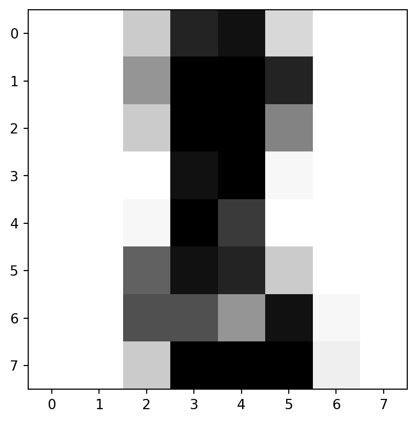
“images”

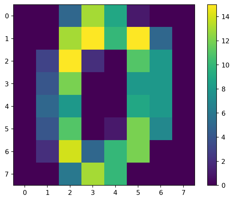
• “images” are more complicated.
• Let’s take a look at just the initial image:

im = digits["images"][0]
im

array([[ 0.,  0.,  5., 13.,  9.,  1.,  0.,  0.],
       [ 0.,  0., 13., 15., 10., 15.,  5.,  0.],
       [ 0.,  3., 15.,  2.,  0., 11.,  8.,  0.],
       [ 0.,  4., 12.,  0.,  0.,  8.,  8.,  0.],
       [ 0.,  5.,  8.,  0.,  0.,  9.,  8.,  0.],
       [ 0.,  4., 11.,  0.,  1., 12.,  7.,  0.],
       [ 0.,  2., 14.,  5., 10., 12.,  0.,  0.],
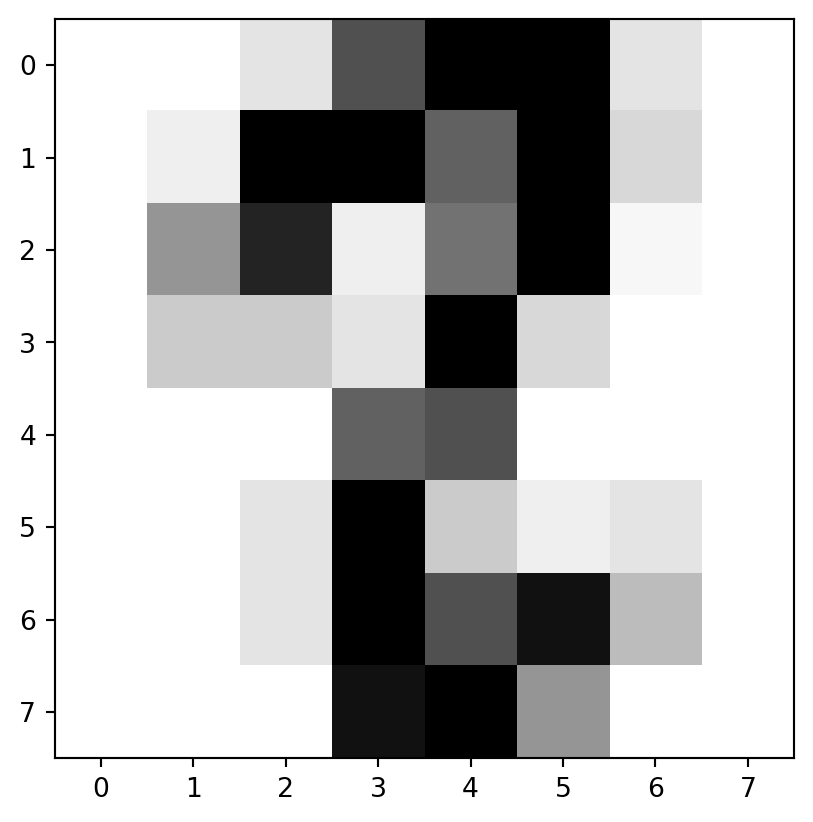
       [ 0.,  0.,  6., 13., 10.,  0.,  0.,  0.]])

Examine

im.shape, im.size, im.ndim

((8, 8), 64, 2)

im.mean(), im.max()

(np.float64(4.59375), np.float64(15.0))

digits["images"].mean(), digits["images"].max()

(np.float64(4.884164579855314), np.float64(16.0))

Takeways

• im is an 8-by-8 array of values from 0 to 16

plt.imshow(im)

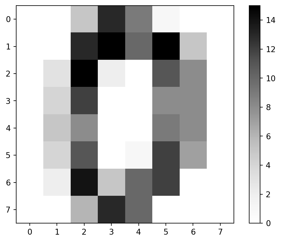
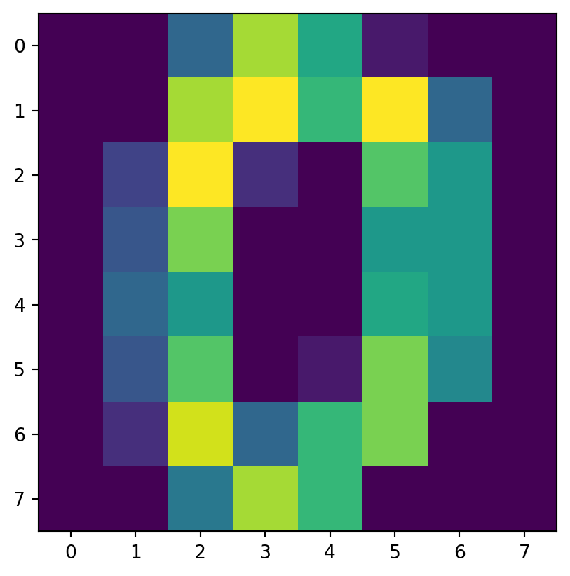
Coloration

plt.imshow(im)
plt.colorbar()

• Might be easier in grayscale.

cmap

• Matplotlib provides colormaps we can specify.
  • I say a 'Greys' in there.

from matplotlib import colormaps
list(colormaps)[:20]

['magma',
 'inferno',
 'plasma',
 'viridis',
 'cividis',
 'twilight',
 'twilight_shifted',
 'turbo',
 'Blues',
 'BrBG',
 'BuGn',
 'BuPu',
 'CMRmap',
 'GnBu',
 'Greens',
 'Greys',
 'OrRd',
 'Oranges',
 'PRGn',
 'PiYG']

Greyscale

plt.imshow(im, cmap='Greys')
plt.colorbar()

Interpolation

• Use an interpolater ('spline16' looked good).

plt.imshow(im) # I am writing a comment here to align vertically

plt.imshow(im, cmap='Greys', interpolation="spline16")

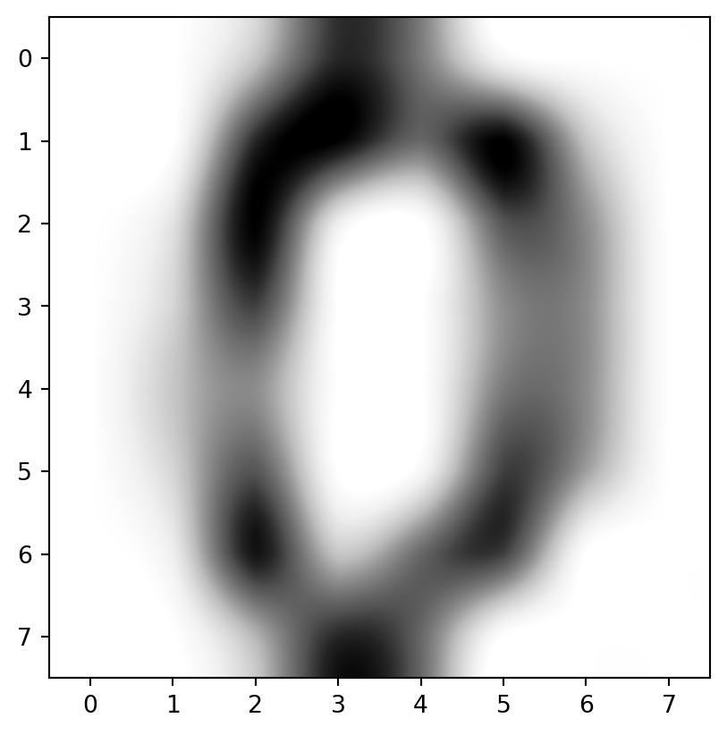
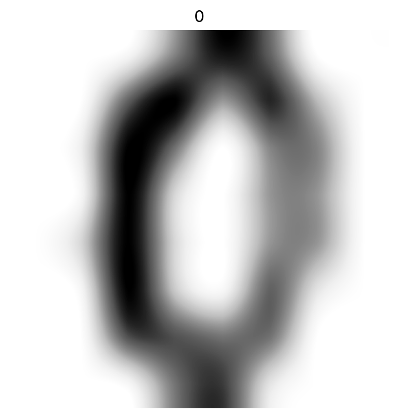
It’s a zero

digits["target"][0]

np.int64(0)

plt.imshow(digits["images"][0], cmap='Greys', interpolation="spline16")

Look at more

• Write a function to check some images out.

def see_im(n):
    plt.imshow(digits["images"][n], cmap='Greys', interpolation='spline16')
    plt.axis('off') # Just looked up how to remove axes
    plt.title(digits["target"][n])
    plt.show() # Like print, for images, or you can save

• Wait how many do I have?

digits["target"].shape

(1797,)

See More

see_im(10)

see_im(100)

see_im(1000)

Classification

Classification

Classification is the activity of assigning objects to some pre-existing classes or categories. This is distinct from the task of establishing the classes themselves (for example through cluster analysis). Examples include diagnostic tests, identifying spam emails and deciding whether to give someone a driving license.

Flatten

• We, as humans, recognize that those things look a lot like images.
• But the images are 3D array, which is more more annoying to work with than one-row-per-digit.
• To begin, we “flatten” to 2D images into 1D arrays.
• We want 1794 arrays of length 64 (was: 8-by-8)

Reshape

• We use NumPy .reshape

count = len(digits["images"])
data = digits["images"].reshape(count, 64)
data[:3]

array([[ 0.,  0.,  5., 13.,  9.,  1.,  0.,  0.,  0.,  0., 13., 15., 10.,
        15.,  5.,  0.,  0.,  3., 15.,  2.,  0., 11.,  8.,  0.,  0.,  4.,
        12.,  0.,  0.,  8.,  8.,  0.,  0.,  5.,  8.,  0.,  0.,  9.,  8.,
         0.,  0.,  4., 11.,  0.,  1., 12.,  7.,  0.,  0.,  2., 14.,  5.,
        10., 12.,  0.,  0.,  0.,  0.,  6., 13., 10.,  0.,  0.,  0.],
       [ 0.,  0.,  0., 12., 13.,  5.,  0.,  0.,  0.,  0.,  0., 11., 16.,
         9.,  0.,  0.,  0.,  0.,  3., 15., 16.,  6.,  0.,  0.,  0.,  7.,
        15., 16., 16.,  2.,  0.,  0.,  0.,  0.,  1., 16., 16.,  3.,  0.,
         0.,  0.,  0.,  1., 16., 16.,  6.,  0.,  0.,  0.,  0.,  1., 16.,
        16.,  6.,  0.,  0.,  0.,  0.,  0., 11., 16., 10.,  0.,  0.],
       [ 0.,  0.,  0.,  4., 15., 12.,  0.,  0.,  0.,  0.,  3., 16., 15.,
        14.,  0.,  0.,  0.,  0.,  8., 13.,  8., 16.,  0.,  0.,  0.,  0.,
         1.,  6., 15., 11.,  0.,  0.,  0.,  1.,  8., 13., 15.,  1.,  0.,
         0.,  0.,  9., 16., 16.,  5.,  0.,  0.,  0.,  0.,  3., 13., 16.,
        16., 11.,  5.,  0.,  0.,  0.,  0.,  3., 11., 16.,  9.,  0.]])

Models

• Foundation to the notion of machine learning is training and testing.
  • More properly to supervised machine learning, but more on that latter.
• Specifically, using training data, we will set the coefficients and parameters of a model, which we can think of as a function with a number of parameters.

Splits

• We split up our data, and
  • Some data we use to train a model.
    • Basically, find coefficients of a function.
  • Some data we use to test a classifier
    • Compare model to actual.

Supervised Learning

Train-Test Split

• The training set is used to teach our model to identify patterns and relationships.
• The testing set is held-out to evaluate the trained model on new, unseen data.

from sklearn.model_selection import train_test_split

X = np.array([[1, 2], [3, 4], [5, 6], [7, 8]])
y = np.array([0, 1, 0, 1])

# Train on 75%, test on 25% by default
X_train, X_test, y_train, y_test = train_test_split(X, y)
X_test, y_test

(array([[1, 2]]), array([0]))

Supervised Learning

• Supervised learning is a type of machine learning where the algorithm learns from labeled data.
• Labeled data consists of input features (X) and corresponding outcomes (y).

from sklearn.linear_model import LinearRegression

# Example labeled data (house size in sqft, price in $1000s)
X_train = np.array([[1000], [1500], [1200], [1800]])
y_train = np.array([200, 300, 240, 360])

model = LinearRegression()
_ = model.fit(X_train, y_train) # The "supervision" happens here

Models and Coefficients

• A model represents the learned relationship inputs-to-targets
• Sometimes this relationship is expressed through coefficients.
• Change in the target a unit change in input feature with other features constant.

# The model learns the equation: price = coefficient * size + intercept
model.coef_, model.intercept_

(array([0.2]), np.float64(-5.684341886080802e-14))

Higher Dimensions

• With multiple input features, each has a coefficient.
• The sign and magnitude of each coefficient show the influence of a feature.

d = {'size': [1000, 1500, 1200, 1800], 'bedrooms': [2, 3, 2, 4], 'price': [200, 300, 240, 360]}
df = pd.DataFrame(d)
X_train, y_train = df[['size', 'bedrooms']], df['price']

model = LinearRegression()
model.fit(X_train, y_train)
model.coef_, model.intercept_

(array([ 2.00000000e-01, -1.32379986e-14]), np.float64(0.0))

The Digits

• We can train/test split the digits like so:

# Recall we "flattened" images into "data"
X_train, X_test, y_train, y_test = train_test_split(data, digits["target"])

Classifiers

Perceptron

• We use a perceptron, one of the oldest and most famous machine learning frameworks.

The artificial neuron network was invented in 1943 by Warren McCulloch and Walter Pitts in A logical calculus of the ideas immanent in nervous activity.

• Described visually in textbooks in 1958
• Inspired by neuroscience ideas of the time.

Import

• Import and create a perceptron.

from sklearn.linear_model import Perceptron
clf = Perceptron() # This will be the model that will contain coefficients
clf # At first, not fitted to anything!

Perceptron()

In a Jupyter environment, please rerun this cell to show the HTML representation or trust the notebook.
On GitHub, the HTML representation is unable to render, please try loading this page with nbviewer.org.

Training

• We train or .fit() the model to the data.

clf.fit(X_train, y_train)

Perceptron()

In a Jupyter environment, please rerun this cell to show the HTML representation or trust the notebook.
On GitHub, the HTML representation is unable to render, please try loading this page with nbviewer.org.

• Then we can predict over the testing set!

y_pred = clf.predict(X_test)
y_pred[:10], y_test[:10]

(array([5, 8, 0, 2, 8, 8, 6, 8, 1, 3]), array([5, 8, 0, 2, 2, 8, 6, 8, 8, 3]))

Not bad!

• More detailed reporting from metrics

from sklearn import metrics

# We print so it looks a bit nicer
print(metrics.classification_report(y_test, y_pred))

              precision    recall  f1-score   support

           0       0.98      0.98      0.98        44
           1       0.83      0.98      0.90        44
           2       1.00      0.95      0.97        39
           3       0.98      0.95      0.97        44
           4       1.00      0.95      0.97        38
           5       0.96      1.00      0.98        51
           6       1.00      0.98      0.99        48
           7       1.00      1.00      1.00        37
           8       0.84      0.92      0.88        63
           9       0.97      0.74      0.84        42

    accuracy                           0.94       450
   macro avg       0.96      0.94      0.95       450
weighted avg       0.95      0.94      0.94       450

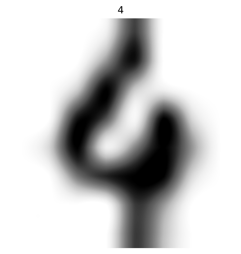
Where did we miss?

• We can see what we got wrong.

# That [0] prevents us from getting tuple of length 1
misses = np.where(y_test != y_pred)[0]
misses

array([  4,   8,  35,  36,  45,  56,  63,  67, 113, 158, 184, 191, 198,
       199, 204, 273, 305, 316, 326, 352, 360, 366, 415, 437, 444])

• Let’s look at the first two of those.

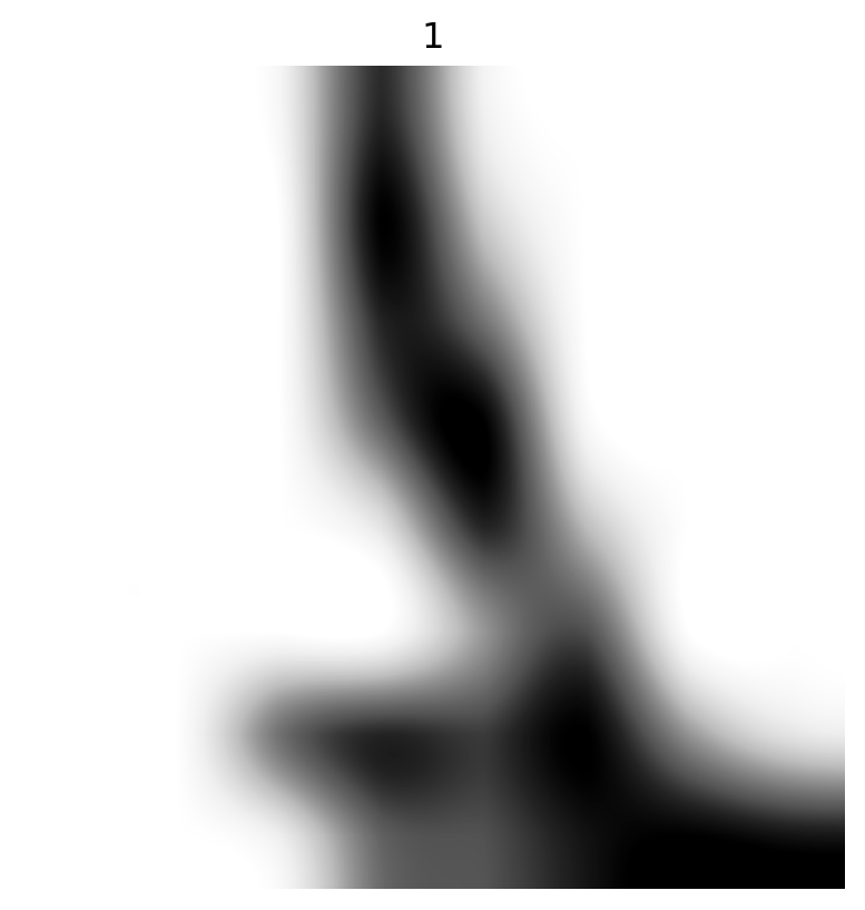
Two Misses

i = misses[0]
print(y_test[i], y_pred[i])
plt.imshow(X_test[i].reshape((8,8)), cmap="Greys")

2 8

i = misses[1]
print(y_test[i], y_pred[i])
plt.imshow(X_test[i].reshape((8,8)), cmap="Greys")

8 1

On Accuracy

• Machine learning frameworks were doing better than I could do around ~2010
• On these older datasets with:
  • Greyscale
  • 16 color
  • 64 pixel
• Maybe your eyes are better than the perceptron, but mine aren’t!

Clustering

Unsupervised Learning

• Unsupervised learning deals with unlabeled data, where there are no predefined target variables (y).
• Find hidden patterns, structures, or relationships within the data itself.

Clustering

• Clustering is an unsupervised learning task that groups data points into clusters based on their similarity.
• Data points within the same cluster are more similar to each other than to those in other clusters.
• The goal is to discover natural groupings in the data without any prior knowledge of those groups.

\(k\)-means Clustering

• \(k\)-means clustering is a popular partitioning algorithm that divides data into k predefined clusters.
• It aims to minimize the sum of squared distances between data points and their assigned cluster’s centroid.
• The k parameter (number of clusters) must be specified in advance.

from sklearn.cluster import KMeans

X = np.array([[1, 2], [1.5, 1.8], [5, 8], [8, 8], [1, 0.6], [9, 11]])
model = KMeans(2) # 2 "clusters"

How \(k\)-means Works

• Start: \(k\) data points as cluster centroids.
• Assign: To the cluster with closest center.
• Update: Recalculate the cluster mean.
• Repeat: Until the assignments no longer change.

# Fit the KMeans model to the data
model.fit(X)
model.cluster_centers_

array([[7.33333333, 9.        ],
       [1.16666667, 1.46666667]])

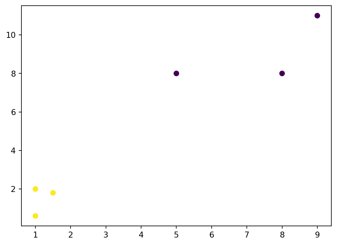
Interpreting \(k\)-means Results

• After fitting, \(k\)-means provides cluster labels for each data point and the coordinates of the cluster centroids.
• The labels indicate which cluster each data point belongs to.
• The centroids represent the “center” of each cluster.

X[model.labels_ == 0]

array([[ 5.,  8.],
       [ 8.,  8.],
       [ 9., 11.]])

X[model.labels_ == 1]

array([[1. , 2. ],
       [1.5, 1.8],
       [1. , 0.6]])

Plot it

x, y = X.transpose()
plt.scatter(x,y,c=model.labels_)

Choosing \(k\)

• Determining the optimal k is a common challenge in \(k\)-means.
• The choice of k often depends on domain knowledge and the goal of the clustering.
• We “cheat” on the digits set - there are 10 digits (exact)

Exercise

Cluster Digits

• For the exercise we will cluster the digits.
• We will use Principle Component Analysis (PCA) to reduce from 64 to fewer dimensions.

Principal Component Analysis

• Dimensionality reduction technique.
• Transforms high-dimensional data into fewer, uncorrelated principal components.
• Components capture maximum data variance.

from sklearn.decomposition import PCA
from sklearn.preprocessing import StandardScaler
X = np.random.rand(50, 5) # 50 samples, 5 features
scaler = StandardScaler()
scaled_X = scaler.fit_transform(X)

PCA: Explained Variance

• Each principal component captures a proportion of the total variance (explained variance ratio).
• Helps decide how many components to keep.

Code Sample

pca = PCA(2)
X_reduced = pca.fit_transform(scaled_X)
X[:5], X_reduced[5]

(array([[0.39250186, 0.86027584, 0.0088714 , 0.09031264, 0.92406155],
        [0.02823733, 0.66593355, 0.91355326, 0.38840791, 0.86576046],
        [0.13334149, 0.67490569, 0.47429288, 0.74461236, 0.62912872],
        [0.45579094, 0.29786937, 0.85740943, 0.08848002, 0.78133508],
        [0.07463008, 0.96488199, 0.27140834, 0.93849056, 0.72967892]]),
 array([-0.80350742, -1.76749167]))

Benefits of PCA

• Simplifies data and reduces storage.
• Can reduce noise.
• Useful for visualization.
• Important: Data scaling is crucial.
  • StandardScaler().fit_transform()

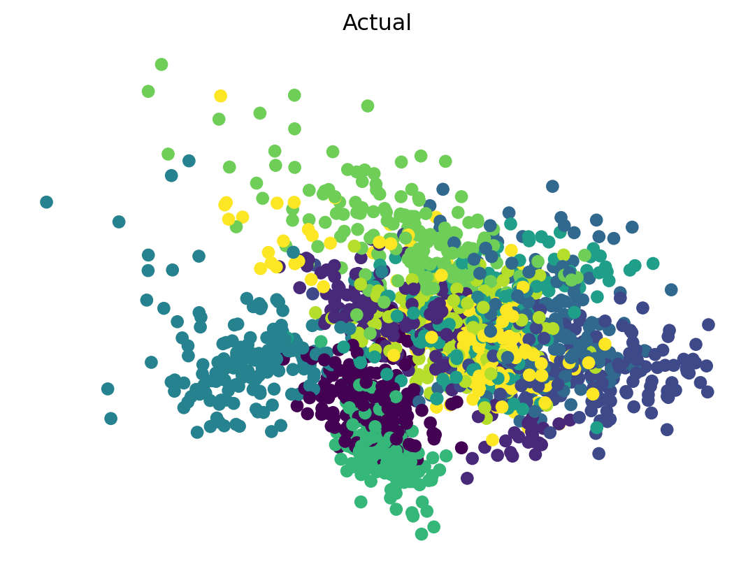
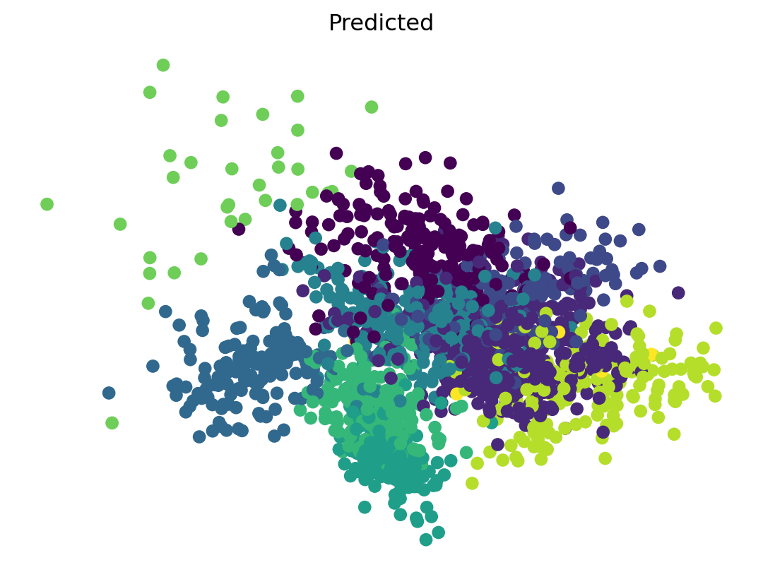
Exercise

• Use PCA and \(k\)-means on the digit data.
  • You may need to try different PCA numbers.
• Look at a 2+ examples in 2+ clusters.
• Plot the classification.
  • I’ll use PCA with 2 dimensions for x and y
  • Two plots, colored for actual and predicted.

Solution

• \(k\)-means

scaled = StandardScaler().fit_transform(data)
reduced = PCA(10).fit_transform(scaled)
model = KMeans(10)
_ = model.fit(reduced)

Looker

• I wrote a function to look at things.

def looker(cluster, index):
    plt.imshow(data[model.labels_ == cluster][index].reshape(8,8), cmap='Greys')
    plt.axis('off')
    plt.show()

Cluster 0

looker(0,0)

looker(0,1)

Cluster 1

looker(1,0)

looker(1,1)

Plot

reduced = PCA(2).fit_transform(scaled)
x, y = reduced.transpose()
plt.scatter(x,y,c=digits["target"])
plt.axis('off') # They are not relative to anything "real"
_ = plt.title("Actual")

reduced = PCA(2).fit_transform(scaled)
x, y = reduced.transpose()
plt.scatter(x,y,c=model.labels_)
plt.axis('off') # They are not relative to anything "real"
_ = plt.title("Predicted")