---
title: Logics
subtitle: "wD"
---
## Announcements
- Last Lecture
- Security topics generally
- Some automata theory
- Action items
- `heap_t` due now
- `BTCinC` final is out
## Today
- Threat and Threat Models
- (Trace) Properties
- Kripke Structures
- Linear Temporal Logic
- Büchi Automata
- DFAs
- Safety & Liveness
- CIA Triad
# Threat
## Threat
- "Security" is incomplete as a concept.
* **What** is secure?
* **For whom** is the 'what' secure?
* **From whom** is the 'what' secure?
## Bitcoin
* **Bitcoins** are secure.
* **For all senders and receivers** the ownership is secured.
* **From any third party** the doublespending is secured.
## Limitations
* Can a third party tell **who** uses the service?
* Can a third party tell **when** coins are being sent?
* Can a third party tell the **amount** of the transaction?
## Models
Use **threat modeling**:
* Description of the subject to be modeled
* Assumptions that can be checked or challenged
* Potential threats to the system
* Actions that can be taken to mitigate each threat
* A way of validating the model and threats
Read more: [OWASP.org](https://owasp.org/www-community/Threat_Modeling)
##
|Informally|Formally|
|-|-|
|**What?**|Description of the subject to be modeled|
|**For whom?**|A way of validating the model and threats|
|**From whom?**|Potential threats to the system|
|**Any limitations?**|Assumptions that can be checked|
|**How?**|Actions that can be taken to mitigate each threat|
## BTC
|Informally|Formally|
|-|-|
|**What?**|Currency|
|**For whom?**|An economy with internet access|
|**From whom?**|Fraud, central authority, surveillance|
|**Any limitations?**|Public ledger|
|**How?**|[bchain.html](bchain.html)|
## How?
We can instead proceed in **four steps**.
1. **Diagram:** What are we building?
1. **Identify threats:** What could go wrong?
1. **Mitigate:** What are we doing to defend against threats?
1. **Validate:** Have we acted on each of the previous steps?
## Diagram
<a style="filter:invert(1)" title="Graingert, CC0, via Wikimedia Commons" href="https://commons.wikimedia.org/wiki/File:Bitcoin_Transaction_Visual.svg"><img width="80%" alt="The mine is closed and the key must stop working. And this key structure has stopped already. by the reason for moving the blueprint and will use the code to confirm the AI service to verify the person instead and generate income into the new..." src="https://upload.wikimedia.org/wikipedia/commons/c/ce/Bitcoin_Transaction_Visual.svg"></a>
## Threats
- What if?
- Two entities have the same private key?
- Dishonest nodes have more compute power?
- Internet goes down?
## Mitigate
- Well...
- Keys are ~4096 bit...
- There are other more lucrative uses of compute than competing with BTC nodes
- If the internet goes down, coins can't be spent but persist locally
## Validate
- This is new!
- Cryptobook uses "Attack Games"
- We explore "digital signature"
## [Cryptobook](https://toc.cryptobook.us/book.pdf):
> We give
the adversary the power to mount a **chosen message attack**, namely the attacker can request the
signature on any message of his choice. Even with such power, the adversary should not be able
to create an **existential forgery**, namely the attacker cannot output a valid message-signature
pair $(m, \omega)$ for some new message $m$.
## [Cryptobook](https://toc.cryptobook.us/book.pdf):
**Attack Game 13.1 (Signature security).** For a given signature scheme $\mathcal{S} = (\mathcal{G}, \mathcal{S}, \mathcal{V})$, (generate, sign, verify) defined over $(\mathcal{M}, \Sigma)$, (messages, signatures), and a given adversary $\mathcal{A}$, the attack game runs as follows:
* The challenger runs $(pk, sk) \leftarrow \mathcal{G}()$ (private signing key, public verifying key) and sends $pk$ to $\mathcal{A}$.
## [Cryptobook](https://toc.cryptobook.us/book.pdf):
**Attack Game 13.1 (Signature security).** For a given signature scheme $\mathcal{S} = (\mathcal{G}, \mathcal{S}, \mathcal{V})$, (generate, sign, verify) defined over $(\mathcal{M}, \Sigma)$, (messages, signatures), and a given adversary $\mathcal{A}$, the attack game runs as follows:
* $\mathcal{A}$ queries the challenger several times. For $i = 1, 2, \dots$, the $i^{th}$ signing query is a message $m_i \in \mathcal{M}$. Given $m_i$, the challenger computes $\sigma_i \leftarrow \mathcal{S}(sk, m_i)$, and then gives $\sigma_i$ to $\mathcal{A}$.
## [Cryptobook](https://toc.cryptobook.us/book.pdf):
**Attack Game 13.1 (Signature security).** For a given signature scheme $\mathcal{S} = (\mathcal{G}, \mathcal{S}, \mathcal{V})$, (generate, sign, verify) defined over $(\mathcal{M}, \Sigma)$, (messages, signatures), and a given adversary $\mathcal{A}$, the attack game runs as follows:
* Eventually $\mathcal{A}$ outputs a candidate forgery pair $(m, \sigma) \in \mathcal{M} \times \Sigma$.
## [Cryptobook](https://toc.cryptobook.us/book.pdf):
**Attack Game 13.1 (Signature security).** For a given signature scheme $\mathcal{S} = (\mathcal{G}, \mathcal{S}, \mathcal{V})$, (generate, sign, verify) defined over $(\mathcal{M}, \Sigma)$, (messages, signatures), and a given adversary $\mathcal{A}$, the attack game runs as follows:
* We say that the adversary wins the game if the following two conditions hold:
$$
\mathcal{V}(pk, m, \sigma) = \text{accept}
$$
## Techniques
* **Define the scope** and depth of analysis.
* Gain a **visual understanding** of what you’re threat modeling.
* Visually **model** the attack possibilities.
* **Identify** threats.
* **Document** of missing or weak security controls.
## Scope
* Determine **stakeholders**
* Who uses the service?
* Who provides the service?
* Who benefits from the service?
* Who does not benefit from the service?
## Scope
* Who can answer these questions?
* Are they the same or different people?
* Should you do this by yourself?
* What do you do if you need help?
## Visuals
```{dot}
//| fig-width: 1000px
//| output-location: slide
//| echo: false
digraph block_chain {
rankdir=TD;
bgcolor="#191919";
node [
fontcolor = "#ffffff",
color = "#ffffff",
shape=record
]
edge [
color = "#ffffff",
fontcolor = "#ffffff"
]
1 [label="{h(prev)|<here> h(root)}|{time|nonce}"]
0 [label="{<there> h(prev)|<here> h(root)}|{time|nonce}"]
2 [label="{<there> h(prev)|<here> h(root)}|{time|nonce}"]
merkle [label="{<1> 0x1|h(*0x2,*0x3)}|{0x2|h(*0x4,*0x5)}|{0x3|h(*0x6,*0x7)}|{0x4|h(*0x8,*0x9)}|{0x5|h(*0xA,*0xB)}|{0x6|<6> h(G,C,2)}|{0x7|<7> h(A,G,4)}|{0x8|<8> h(A,B,1)}|{0x9|<9> h(B,C,2)}|{0xA|<A> h(C,D,3)}|{0xB|<B> h(F,A,7)}"]
heap [shape=record, label="{send|recv|amnt}|{<e> G|C|2}|{<f> A|G|4}|{<a> A|B|1}|{<b> B|C|2}|{<c> C|D|3}|{<d> F|A|7}"]
1 -> 0:there
0 -> merkle:1
0 -> 2:there
merkle:7 -> heap:f
merkle:6 -> heap:e
merkle:B -> heap:d
merkle:A -> heap:c
merkle:9 -> heap:b
merkle:8 -> heap:a
}
```
## Threats
* What if?
- Someone changes `(G,C,2)` to `(G,C,3)`
- `G` submits a second `(G,G,2)` next block
- `G` loses their private key?
## Document
- [https://bitcoin.org/bitcoin.pdf](https://bitcoin.org/bitcoin.pdf)
- [https://github.com/bitcoin/bitcoin](https://github.com/bitcoin/bitcoin)
## **Traffic light**
* **Diagram:** What are we building?
* **Identify threats:** What could go wrong?
* **Mitigate:** What are we doing to defend against threats?
* **Validate:** Have we acted on each of the previous steps?
## Today
- ✓ Threat and Threat Models
- (Trace) Properties
- Kripke Structures
- Linear Temporal Logic
- Büchi Automata
- DFAs
- Safety & Liveness
- CIA Triad
# Properties
## Properties
* A **security policy** may have **properties**.
* These **security policies** are distinct from the **what?** of a threat model
* Rather the **security policy** is the **how?** of a threat model
A security policy could have the property of being **secure** if the threats of a threat model are mitigated
## Trace Properties
* I think of properties in terms of **traces**
* A **trace** is the sequence of states through which a system passes over time.
* A **sequence** is an ordered collection.
* A **state** is the configuration of a system at some specific time point.
* A **system** implements the security policy.
* Emphasize the notion of **over time**. Traces are **time-based**.
## Traffic Light
* Think of a **traffic light**.
* In what **states** may a traffic light be?
* In what **sequence** may these states occur?
* Does a traffic light implement a **security policy**
* Do traffic lights **change over time**?
## State Machine
- A traffic light is a **state machine**.
> [A **state machine** is a mathematical model of computation. It is an abstract machine that can be in exactly one of a finite number of states at any given time.](https://en.wikipedia.org/wiki/Finite-state_machine)
- Often called "FSM" (finite state machine)
- I don't have a hot new start-up selling infinite states.
## A Trace
- We can denote the state of a traffic light by the lit color. ("Wow this class is lit.")
- A trace may appear as:
```{.python}
trace = [
    "RED___",
    "GREEN_",
    "YELLOW",
    "RED___",
    "GREEN_",
    "YELLOW",
    "RED___",
    "GREEN_",
    "YELLOW"
]
```
## Examples
- Let's review some traces and see if they are from a traffic light system that is operating properly.
```{.python}
summarize = lambda t : "".join([s[0] for s in t])
```
- Can also express traces as e.g. `RGYRGYRGY`
## Start
- Does **starting state** matter?
::::{columns}
:::{.column width=33%}
```{.python}
trace = [
    "YELLOW",
    "RED___",
    "GREEN_",
    "YELLOW",
    "RED___",
    "GREEN_",
    "YELLOW"
]
```
:::
:::{.column width=33%}
```{.python}
trace = [
    "GREEN_",
    "YELLOW",
    "RED___",
    "GREEN_",
    "YELLOW",
    "RED___",
    "GREEN_"
]
```
:::
:::{.column width=33%}
```{.python}
trace = [
    "RED___",
    "GREEN_",
    "YELLOW",
    "RED___",
    "GREEN_",
    "YELLOW",
    "RED___"
]
```
:::
::::
## End
- Does **ending state** (terminating state) matter?
::::{columns}
:::{.column width=33%}
```{.python}
trace = [
    "YELLOW",
    "RED___",
    "GREEN_",
    "YELLOW",
    "RED___",
    "GREEN_",
    "YELLOW"
]
```
:::
:::{.column width=33%}
```{.python}
trace = [
    "GREEN_",
    "YELLOW",
    "RED___",
    "GREEN_",
    "YELLOW",
    "RED___",
    "GREEN_"
]
```
:::
:::{.column width=33%}
```{.python}
trace = [
    "RED___",
    "GREEN_",
    "YELLOW",
    "RED___",
    "GREEN_",
    "YELLOW",
    "RED___"
]
```
:::
::::
## Length
- Does **length** (or perhaps size) matter?
::::{columns}
:::{.column width=33%}
```{.python}
trace = [
    "YELLOW",
    "RED___"
]
```
:::
:::{.column width=33%}
```{.python}
trace = [
    "GREEN_",
    "YELLOW",
    "RED___",
    "GREEN_",
    "YELLOW"
]
```
:::
:::{.column width=33%}
```{.python}
trace = [
    "RED___",
    "GREEN_",
    "YELLOW",
    "RED___",
    "GREEN_",
    "YELLOW",
    "RED___"
]
```
:::
::::
## Unique
- Does **number of unique states** matter?
::::{columns}
:::{.column width=33%}
```{.python}
trace = [
    "YELLOW",
]
```
:::
:::{.column width=33%}
```{.python}
trace = [
    "GREEN_",
    "YELLOW"
]
```
:::
:::{.column width=33%}
```{.python}
trace = [
    "RED___",
    "GREEN_",
    "YELLOW"
]
```
:::
::::
## Order
- Does **order** matter?
::::{columns}
:::{.column width=33%}
```{.python}
trace = [
    "GREEN_",
    "RED___",
    "YELLOW"
]
```
:::
:::{.column width=33%}
```{.python}
trace = [
    "RED___",
    "YELLOW",
    "GREEN_"
]
```
:::
:::{.column width=33%}
```{.python}
trace = [
    "RED___",
    "GREEN_",
    "YELLOW"
]
```
:::
::::
## Sets of Traces
::: {.callout-note}
A **trace property** is a set of traces.
:::
- Say, variable "property" is a list of traces.
- *Should* be a set.
```{.py}
property[0] = ["GREEN_"]
property[1] = ["YELLOW"]
property[2] = ["RED___"]
property[3] = ["GREEN_", "YELLOW"]
```
## System Properties
* Say a system "satisfies" property $p$ if all possible traces produced by a system are in the property.
* This may be an infinite number of traces or include traces of infinite length.
* Systems may have (satisfy) more than one property.
## On Security
Properties provide a way to answer the "How?" after asking:
* **What** is secure?
* **For whom** is the 'what' secure?
* **From whom** is the 'what' secure?
## Sets of Traces
- A **set** is an ordered collection of elements (such as sequences).
- A **sequence** is an ordered collection of elements (such as states).
- A **trace property** is a set of traces.
- A **trace** is a sequence of states.
## Organization
```{dot}
//| echo: false
//| fig-width: 1000px
digraph PropertyHierarchy {
bgcolor="#191919";
node [shape=box, style=rounded, fontcolor=white, color=white];
edge [color=white];
PROPERTY [label="PROPERTY\nSet of traces"];
SET [label="SET\nUnordered elements"];
TRACE [label="TRACE\nSequence of states"];
SEQUENCE [label="SEQUENCE\nOrdered elements"];
STATES [label="STATES\nDescribe a system at\nsome time"];
PROPERTY -> SET;
PROPERTY -> TRACE;
TRACE -> SEQUENCE;
TRACE -> STATES;
}
```
## Example
```{dot}
//| echo: false
//| fig-width: 1000px
digraph PropertyHierarchy {
bgcolor="#191919";
node [shape=box, style=rounded, fontcolor=white, color=white];
edge [color=white];
PROPERTY [label="PROPERTY\n{R,YR,GYR,RGYR}"];
SET [label="SET\nUnordered elements"];
TRACE [label="TRACE\nRGYR"];
SEQUENCE [label="SEQUENCE\nOrdered elements"];
STATES [label="STATES\n{RED___, GREEN_}"];
PROPERTY -> SET;
PROPERTY -> TRACE;
TRACE -> SEQUENCE;
TRACE -> STATES;
}
```
## Enumeration
- Thus far, we enumerated the possible traces.
```{.python}
property[0] = ["GREEN_"]
property[1] = ["YELLOW"]
property[2] = ["RED___"]
property[3] = ["GREEN_", "YELLOW"]
```
- This is bad. Why?
## Specification
- Rather than enumerate, let us specify.
```{.email}
The traffic light property is
    the set of all sequences over precisely the states {"GREEN_", "YELLOW", "RED___"} such that
        the only state succeeding "GREEN_" is "YELLOW" and
        the only state succeeding "YELLOW" is "RED___" and
        the only state succeeding "RED___" is "GREEN_".
```
## Today
- ✓ Threat and Threat Models
- ✓ (Trace) Properties
- Kripke Structures
- Linear Temporal Logic
- Büchi Automata
- DFAs
- Safety & Liveness
- CIA Triad
# Kripke Structures
## Model Checking
- A Kripke Structure is a tuple that models a state machine.
- Recall:
- A **state machine** is a mathematical model of computation. It is an abstract machine that can be in exactly one of a finite number of states at any given time.
- Exactly one!
## Model Checking
A Kripke Structure is a tuple {_S_, ...} that models a state machine.
* _S_ is a finite set of states
* Kripke structures only work for **finite** state machines
* For the sake of this class, we can imagine infinite states if needed.
## Model Checking
A Kripke Structure is a tuple {_S_, ...} that models a state machine.
* For a traffic light, _S_ is:
`{"GREEN_", "YELLOW", "RED___"}`
* For a Bitcoin, it is perhaps the current owner.
* Many possible, but finite, number of owners.
## Model Checking
A Kripke Structure is a tuple {_S_, _I_, ...} that models a state machine.
* _I_ is a subset of _S_, we denote this _I_ ⊂ _S_
* Any state in _I_ must be a state in _S_
* There may be states in _S_ that are not in _I_
* These are the possible initial states of the state machine.
## Model Checking
A Kripke Structure is a tuple {_S_, _I_, ...} that models a state machine.
* For a traffic light, _I_ = _S_ `{"GREEN_", "YELLOW", "RED___"}`
* For a Bitcoin, the initial state is Satoshi Nakamoto's public key.
## Model Checking
A Kripke Structure is a tuple {_S_, _I_, ...} that models a state machine.
* _S_ is a finite set of states
* _I_ ⊂ _S_ is the set of initial states.
## Model Checking
A Kripke Structure is a tuple {_S_, _I_, _R_, ...} that models a state machine.
* _R_ is a **transition relation** over _S_, we denote this _R_ ⊂ _S_ × _S_
* This just means _R_ says whether one state may be transitioned to from another.
* Same as graph edges (if we take _S_ to be nodes)
## Model Checking
* **BONUS/CHALLENGE:** _R_ is left-total.
:::{.callout-note}
A binary relation _R_ ⊂ _S_ × _S_ is **left-total** if for all elements _s_ of _S_ there exists some ordered pair in _R_ such that the first element of the ordered pair is _s_.
:::
* _R_ ⊂ _S_ × _S_ is **left-total** ≔ ∀ _s1_ ∈ _S_, ∃ _s2_ ∈ _S_ such that (_s1_,_s2_) ∈ _R_
## Model Checking
A Kripke Structure is a tuple {_S_, _I_, _R_, ...} that models a state machine.
* For a traffic light, _R_ is:
```{.py}
{("GREEN_", "YELLOW"),
 ("YELLOW", "RED___"),
 ("RED___", "GREEN_")}
```
* For Bitcoin, the Cartesian product.
## Model Checking
A Kripke Structure is a tuple {_S_, _I_, _R_, ...} that models a state machine.
* _S_ is a finite set of states
* _I_ ⊂ _S_ is the set of initial states.
* _R_ ⊂ _S_ × _S_ is a left-total transition relation.
## Model Checking
A Kripke Structure is a 4-tuple {_S_, _I_, _R_, _L_} that models a state machine.
* _L_ is a **labeling function** over _S_, we denote this _L_ ⊂ _S_ → ???
* This just means _L_ provides a way of talking about the states in _S_
* We talk about these states using **atomic propositions**
## Atomic Propositions
* Propositions are expressions in propositional, or zeroth order, logic.
* They are simply true or false.
* Atomic propositions are simplest possible form of these logic expressions.
* _L_ ⊂ _S_ → 2<sup>_AP_</sup>
## Model Checking
A Kripke Structure is a 4-tuple {_S_, _I_, _R_, _L_} that models transitions between over atomic propositions _AP_.
* _L_ is a **labeling function** over _S_, we denote this _L_ ⊂ _S_ → 2_AP_
* Given _AP_, _L_ tells us whether each is `true` or `false` (2 options) for every given state.
## Model Checking
A Kripke Structure is a 4-tuple {_S_, _I_, _R_, _L_} that models transitions and _AP_.
* For a traffic light, regard _AP_ as the bit encoding of the current state, with perhaps bits encoding "redness", "yellowness", and "greenness"
* These happen to be but are not required to be mutually exclusive.
## AP
* Or just take a "red" and "green" proposition.
* The easiest way to imagine this is with hexcodes
```{.python}
red    = 0xFF0000
green  = 0x00FF00
yellow = red + green
```
* Regard a yellow light as a light that is both red and green (after all... it is)
## Model Checking
A Kripke Structure is a 4-tuple {_S_, _I_, _R_, _L_} that models transitions and _AP_.
* _S_ is a finite set of states
* _I_ ⊂ _S_ is the set of initial states.
* _R_ ⊂ _S_ × _S_ is a left-total transition relation.
* _L_ ⊂ _S_ → 2_AP_ is the labelling relation.
<!--
Model Checking
--------------
A Kripke Structure is a 4-tuple {_S_, _I_, _R_, _L_} that models transitions and _AP_.
* _S_ is a finite set of states and _I_ ⊂ _S_ is the set of initial states.
{"GREEN_", "YELLOW", "RED___"}
* _R_ ⊂ _S_ × _S_ is a left-total transition relation.
{("GREEN_", "YELLOW"),
("YELLOW", "RED___"),
("RED___", "GREEN_")}
* _L_ ⊂ _S_ → 2_AP_ is the labelling relation.
{("GREEN_", {p, s, u}),
("YELLOW", {q, s, t}),
("RED___", {r, t, u})}
A Kripke Structure modelling a traffic light is the 4-tuple...
({"GREEN_", "YELLOW", "RED___"},
{"GREEN_", "YELLOW", "RED___"},
{("GREEN_", "YELLOW"),
("YELLOW", "RED___"),
("RED___", "GREEN_")},
{("GREEN_", {p, s, u}),
("YELLOW", {q, s, t}),
("RED___", {r, t, u})})
...over _AP_...
[p : state == "GREEN_",
q : state == "YELLOW",
r : state == "RED___",
s : state ∈ {"GREEN_", "YELLOW"},
t : state ∈ {"YELLOW", "RED___"},
u : state ∈ {"RED___", "GREEN_"}]
Model Checking
--------------
A Kripke Structure is a 4-tuple {_S_, _I_, _R_, _L_} that models transitions and _AP_.
* This is still bad. Why?
-->
## Diagrams
Now that I've rigorously defined Kripke Structures, I am willing to tell you they are just diagrams.
* Clarke, Edmund & Grumberg, Orna & Jha, Somesh & Lu, Yuan & Veith, Helmut. (2003). Counterexample-guided abstraction refinement for symbolic model checking. J. ACM. 50. 752-794. 10.1145/876638.876643.
## Diagrams
::::{columns}
:::{.column width=50%}
- $\{S, I, R, L\}$
- $S := \{ S_1, S_2, S_3 \}$
- $I := \{ S_1 \}$
- $R := \{(1,2), (2,1), (2,3), (3,3)\}$
- $L := \{({p,q},1), ({q},2), ({p},3)\}$
:::
:::{.column width=50%}
<a style="filter:invert(1)" title="Original file: Ashutosh y0078
Updated version: Ixfd64, CC BY 3.0 <https://creativecommons.org/licenses/by/3.0>, via Wikimedia Commons" href="https://commons.wikimedia.org/wiki/File:KripkeStructureExample.svg"><img width="100%" alt="KripkeStructureExample" src="https://upload.wikimedia.org/wikipedia/commons/3/3b/KripkeStructureExample.svg"></a>
:::
::::
## Traffic Light
::::{columns}
:::{.column width=50%}
- $\{S, I, R, L\}$
:::
:::{.column width=50%}
```{dot}
//| fig-width: 400px
//| echo: false
digraph block_chain {
rankdir=TD;
bgcolor="#191919";
node [
fontcolor = "#ffffff",
color = "#ffffff",
shape=circle
]
edge [
color = "#ffffff",
fontcolor = "#ffffff"
]
}
```
:::
::::
## Traffic Light
::::{columns}
:::{.column width=50%}
- $\{S, I, R, L\}$
- $S := \{ S_1, S_2, S_3 \}$
- Denote states as numbered circles.
:::
:::{.column width=50%}
```{dot}
//| fig-width: 400px
//| echo: false
digraph block_chain {
rankdir=TD;
bgcolor="#191919";
node [
fontcolor = "#ffffff",
color = "#ffffff",
shape=circle
]
edge [
color = "#ffffff",
fontcolor = "#ffffff"
]
1 [label=<S<SUB>1</SUB>>]
2 [label=<S<SUB>2</SUB>>]
3 [label=<S<SUB>3</SUB>>]
}
```
:::
::::
## Traffic Light
::::{columns}
:::{.column width=50%}
- $\{S, I, R, L\}$
- $S := \{ S_1, S_2, S_3 \}$
- $I := \{ S_1, S_2, S_3 \}$
- Denote as incoming arrows
:::
:::{.column width=50%}
```{dot}
//| fig-width: 400px
//| echo: false
digraph block_chain {
rankdir=TD;
bgcolor="#191919";
node [
fontcolor = "#ffffff",
color = "#ffffff",
shape=circle
]
edge [
color = "#ffffff",
fontcolor = "#ffffff"
]
01 [label="", shape=point]
1 [label=<S<SUB>1</SUB>>]
01 -> 1
02 [label="", shape=point]
2 [label=<S<SUB>2</SUB>>]
02 -> 2
03 [label="", shape=point]
3 [label=<S<SUB>3</SUB>>]
03 -> 3
}
```
:::
::::
## Traffic Light
::::{columns}
:::{.column width=50%}
- $\{S, I, R, L\}$
- Skip to labels
- Basically have:
- $\{r\}$
- $\{g\}$
- $\{r,g\}$
- Just use that order.
:::
:::{.column width=50%}
```{dot}
//| fig-width: 400px
//| echo: false
digraph block_chain {
rankdir=TD;
bgcolor="#191919";
node [
fontcolor = "#ffffff",
color = "#ffffff",
shape=circle
]
edge [
color = "#ffffff",
fontcolor = "#ffffff"
]
01 [label="", shape=point]
1 [label=<S<SUB>1</SUB><br/><br/>{ r }>]
01 -> 1
02 [label="", shape=point]
2 [label=<S<SUB>2</SUB><br/><br/>{ g }>]
02 -> 2
03 [label="", shape=point]
3 [label=<S<SUB>3</SUB><br/><br/>{r,g}>]
03 -> 3
}
```
:::
::::
## Traffic Light
::::{columns}
:::{.column width=50%}
- $\{S, I, R, L\}$
- The state names are not meaningful
- I can make them whatever I want via $L$
:::
:::{.column width=50%}
```{dot}
//| fig-width: 400px
//| echo: false
digraph block_chain {
rankdir=TD;
bgcolor="#191919";
node [
fontcolor = "#ffffff",
color = "#ffffff",
shape=circle
]
edge [
color = "#ffffff",
fontcolor = "#ffffff"
]
01 [label="", shape=point]
1 [label=<R<br/>{ r }>]
01 -> 1
02 [label="", shape=point]
2 [label=<G<br/>{ g }>]
02 -> 2
03 [label="", shape=point]
3 [label=<Y<br/>{r,g}>]
03 -> 3
}
```
:::
::::
## Traffic Light
::::{columns}
:::{.column width=50%}
- $\{S, I, R, L\}$
- We have our transition relation.
- Side-to-top
||R|G|Y|
|-|-|-|-|
|R||x||
|G|||x|
|Y|x|||
:::
:::{.column width=50%}
```{dot}
//| fig-width: 400px
//| echo: false
digraph block_chain {
rankdir=LR;
bgcolor="#191919";
node [
fontcolor = "#ffffff",
color = "#ffffff",
shape=circle
]
edge [
color = "#ffffff",
fontcolor = "#ffffff"
]
1 [label=<R<br/>{ r }>]
2 [label=<G<br/>{ g }>]
3 [label=<Y<br/>{r,g}>]
1 -> 2
2 -> 3
3 -> 1
01 [label="", shape=point]
02 [label="", shape=point]
03 [label="", shape=point]
02 -> 2
01 -> 1
03 -> 3
}
```
:::
::::
## Traffic Light
::::{columns}
:::{.column width=50%}
- $\{S, I, R, L\}$
- Perhaps omit $I$ denotation.
:::
:::{.column width=50%}
```{dot}
//| fig-width: 400px
//| echo: false
digraph block_chain {
rankdir=TD;
bgcolor="#191919";
node [
fontcolor = "#ffffff",
color = "#ffffff",
shape=circle
]
edge [
color = "#ffffff",
fontcolor = "#ffffff"
]
1 [label=<R<br/>{ r }>]
3 [label=<Y<br/>{r,g}>]
2 [label=<G<br/>{ g }>]
3 -> 1
2 -> 3
1 -> 2
}
```
:::
::::
## Acceptance
::::{columns}
:::{.column width=50%}
- We say a trace is accepted if
- It starts in a start state, and
- For each new tracepoint, there is an edge.
:::
:::{.column width=50%}
```{dot}
//| fig-width: 400px
//| echo: false
digraph block_chain {
rankdir=TD;
bgcolor="#191919";
node [
fontcolor = "#ffffff",
color = "#ffffff",
shape=circle
]
edge [
color = "#ffffff",
fontcolor = "#ffffff"
]
1 [label=<R<br/>{ r }>]
3 [label=<Y<br/>{r,g}>]
2 [label=<G<br/>{ g }>]
3 -> 1
2 -> 3
1 -> 2
}
```
:::
::::
## Acceptance
::::{columns}
:::{.column width=50%}
- `R` is accepted.
:::
:::{.column width=50%}
```{dot}
//| fig-width: 400px
//| echo: false
digraph block_chain {
rankdir=TD;
bgcolor="#191919";
node [
fontcolor = "#ffffff",
color = "#ffffff",
shape=circle
]
edge [
color = "#ffffff",
fontcolor = "#ffffff"
]
1 [label=<R<br/>{ r }>]
3 [label=<Y<br/>{r,g}>]
2 [label=<G<br/>{ g }>]
0 [label="", shape="point"]
0 -> 1 [color = "#ffa07a"]
3 -> 1
2 -> 3
1 -> 2
}
```
:::
::::
## Acceptance
::::{columns}
:::{.column width=50%}
- `RG` is accepted.
:::
:::{.column width=50%}
```{dot}
//| fig-width: 400px
//| echo: false
digraph block_chain {
rankdir=TD;
bgcolor="#191919";
node [
fontcolor = "#ffffff",
color = "#ffffff",
shape=circle
]
edge [
color = "#ffffff",
fontcolor = "#ffffff"
]
1 [label=<R<br/>{ r }>]
3 [label=<Y<br/>{r,g}>]
2 [label=<G<br/>{ g }>]
0 [label="", shape="point"]
0 -> 1 [color = "#ffa07a"]
3 -> 1
2 -> 3
1 -> 2 [color = "#ffa07a"]
}
```
:::
::::
## Rejection
::::{columns}
:::{.column width=50%}
- `RY` is a rejected.
- No edge from `R` to `Y`
:::
:::{.column width=50%}
```{dot}
//| fig-width: 400px
//| echo: false
digraph block_chain {
rankdir=TD;
bgcolor="#191919";
node [
fontcolor = "#ffffff",
color = "#ffffff",
shape=circle
]
edge [
color = "#ffffff",
fontcolor = "#ffffff"
]
1 [label=<R<br/>{ r }>]
3 [label=<Y<br/>{r,g}>]
2 [label=<G<br/>{ g }>]
0 [label="", shape="point"]
0 -> 1 [color = "#ffa07a"]
3 -> 1
2 -> 3
1 -> 2
1 -> 3 [style="dashed", color="red"]
}
```
:::
::::
<!--
Diagrams
--------
A Kripke Structure is a 4-tuple {_S_, _I_, _R_, _L_}
* _S_ is the states, in blue.
Diagrams
--------
A Kripke Structure is a 4-tuple {_S_, _I_, _R_, _L_}
* _S_ is the states, in blue.
* _I_ is the inital states, in orange.
* _R_ is the relations, in purple.
Diagrams
--------
A Kripke Structure is a 4-tuple {_S_, _I_, _R_, _L_}
* _S_ is the states, in blue.
* _I_ is the inital states, in orange.
* _R_ is the relations, in purple.
* _L_ is the labels, in black.
-->
## Limitations
- Better than enumeration, but...
* In text is too complex
* Considering traces is difficult in nontrivial cases.
- We will introduce a better way to write out relations, then look at our Kripke Structures.
## TCP
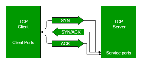
- Consider the "famous" TCP 3-way handshake.
<img src="https://media.geeksforgeeks.org/wp-content/uploads/handshake-1.png" style="filter:invert(.9)">
- [More](https://www.geeksforgeeks.org/tcp-3-way-handshake-process/)
## TCP
::::{columns}
:::{.column width=50%}
- State is more complex.
- Tracking whether `SYN` and `ACK` have been received by both client and server.
:::
:::{.column width=50%}
<img src="https://media.geeksforgeeks.org/wp-content/uploads/handshake-1.png" style="filter:invert(.9)">
:::
::::
## TCP
::::{columns}
:::{.column width=50%}
- Transitions are more complex.
- Vs, a light which *is* red and *becomes* red.
- A server *is* in state, say `LISTEN` and then transitions to state `SYN-RECEIVED`.
:::
:::{.column width=50%}
<img src="https://media.geeksforgeeks.org/wp-content/uploads/handshake-1.png" style="filter:invert(.9)">
:::
::::
## TCP
::::{columns}
:::{.column width=50%}
- Is this trace accepted?
1. `Client.SYN`
2. `Client.SYN` x2
3. `Server.SYN`
4. `Server.ACK`
5. `Client.ACK`
:::
:::{.column width=50%}
<img src="https://media.geeksforgeeks.org/wp-content/uploads/handshake-1.png" style="filter:invert(.9)">
:::
::::
<!--
A concretization
----------------
Consider the following representation:
* Take `p` to be "password checking is blocked/secured"
* Take `q` to be "system access is blocked/secured"
A passwording service **must** disclose if an entered password is correct.
* `p` and `q` are true initially.
* No checking, no access
* Once `q` becomes false, it never becomes true again.
* Once logged in, we can no longer guess passwords.
* Once `q` becomes false, `p` stays true forever.
* Once logged in, access is not revoked.
Infinite guesses (bad), but persistent users may not look up passwords (good).
Goals
-----
We have:
* A way to describe the current state of the system (_AP_)
We need:
* A way to describe relations between atomic propositions over time.
Consider:
* `p` and `q` are true **initially**.
* Once `q` becomes false, it never becomes true again.
* `q` until not `q`
* Once `q` becomes false, `p` stays true forever.
* `q` until not `q`
* `p` goes from false to true when `q` goes from true to true false.
-->
## TCP
::::{columns}
:::{.column width=50%}
* Server/Client requires `SYN` initially.
* Server may not 'SYN' or `ACK` until seeing `SYN`
* Client may not `ACK` until seeing `ACK`
* Client must `ACK`
:::
:::{.column width=50%}
<img src="https://media.geeksforgeeks.org/wp-content/uploads/handshake-1.png" style="filter:invert(.9)">
:::
::::
## Today
- ✓ Threat and Threat Models
- ✓ (Trace) Properties
- ✓ Kripke Structures
- Linear Temporal Logic
- Büchi Automata
- DFAs
- Safety & Liveness
- CIA Triad
# LTL
## neXt and Until
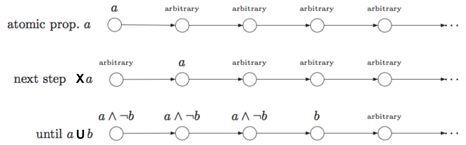
- It often suffices to define two temporal operators:
* **X**: “neXt”
* **U**: “Until”
- Along with existing logical operators:
* **¬**: “not”
* **∨**: “or”
- Apply these over atomic propositions in _AP_ to describe security.
## Composition
With logical negation (not) and disjunction (or) we can generate other logical connectives.
| $p$ | $q$ | $\neg p$ | $p \lor q$ | $\neg p \lor \neg q$ | $\neg p \lor \neg q \equiv p \land q$ |
| :---- | :---- | :---- | :---- | :---- | :------------ |
| True | True | False | True | False | True |
| True | False | False | True | True | False |
| False | True | True | True | True | False |
| False | False | True | False | True | False |
## Next and Until
<img src="https://cd-public.github.io/courses/old/secs24/slides/images/xu.png" style="filter:invert(.9)">
## Derived Unary
| Name | Written: | Meaning | Equivalencies |
| :------------- | :------------ | :------------------------------------------------------------------------- | :---------------------------- |
| neXt | **X** _p_ | _p_ holds in the next time | **X** _p_ |
| Future | **F** _p_ | _p_ holds in some future time | True **U** _p_ |
| Global(ly) | **G** _p_ | _p_ holds future times | **¬**(True **U** **¬** _p_) |
## Derived Binary
| Name | Written: | Meaning | Equivalencies |
| :------------- | :------------ | :------------------------------------------------------------------------- | :---------------------------- |
| Until | _p_ **U** _q_ | _p_ holds unless _q_, _q_ must hold eventually | _p_ **U** _q_ |
| Release | _p_ **R** _q_ | _q_ holds up to and including when _p_ holds | **¬**(**¬** _p_ **U** **¬** _q_) |
## Special Binary
| Name | Written: | Meaning | Equivalencies |
| :------------- | :------------ | :------------------------------------------------------------------------- | :---------------------------- |
| Weak until | _p_ **W** _q_ | _p_ holds up to when _q_ holds | (_p_ **U** _q_) ∨ **G** _p_ |
| Mighty release | _p_ **M** _q_ | _q_ holds up to and including when _p_ holds, and _p_ must hold eventually | _q_ **U** (_p_ **∨** _q_) |
## Properties
* Some security properties are about bad things not happening:
* **G** $\neg$ _bad_
* Term this "safety"
* Some security properties are about good things happening someday:
* **F** _good_
* Term this "liveness"
## Today
- ✓ Threat and Threat Models
- ✓ (Trace) Properties
- ✓ Kripke Structures
- ✓ Linear Temporal Logic
- Büchi Automata
- DFAs
- Safety & Liveness
- CIA Triad
# Automata
## Aside
- Büchi Automata are just "DFA" (deterministic finite automata) that aren't finite.
- They accomplish this through an uninteresting hack.
- DFAs are the first automata taught in theory of computing and automata theory class.
- The follow slides conclude the "sets/graphs/automata" portion of class, among other things.
<!--
Büchi Automata
--------------
* Logicians use Büchi Automata to define **safety** and **liveness** more formally.
* Büchi Automata are more expressive than Kripke Structures
* Deterministic Büchi Automata are equivalent to LTL
* What would it mean for a Kripke Structure to be deterministic?
* What would it mean for LTL not to be deterministic?
## Büchi Automata
A deterministic Büchi Automaton either accepts or rejects infinite inputs (traces).
## Büchi Automata
A deterministic Büchi Automaton _A_ is a tuple {_Q_, ...} that accepts traces.
* _Q_ is a finite set.
* We term the elements of _Q_ to be the states of _A_
* The states of _A_ may be distinct from the unique states found within a trace.
* Traces of infinite length can be considered.
* _Q_ is circles in our diagram.
Büchi Automata
--------------
A deterministic Büchi Automaton _A_ is a tuple {_Q_, _Σ_,...} that accepts traces.
* _Σ_ (sigma) is a finite set.
* We term _Σ_ the alphabet of _A_
* _Σ_ is the unique states found within a trace.
* We use _Σ_ ω (upper case sigma raised to lower case omega) to denote infinite traces
* These are the possible states of a trace; I term them letters.
Büchi Automata
--------------
A deterministic Büchi Automaton _A_ is a tuple {_Q_, _Σ_,...} that accepts traces _Σ_ ω.
* _Q_ is a finite set: the states of _A_.
* _Σ_ is a finite set: the alphabet of _A_.
We studied example traces earlier, for these:
Σ = { {'p', 'q'}, {'p'}, {'q'} }
We cannot yet generate something that looks like _Q_, but it is similar to
Q ≈ {'s_1', 's_2', 's_3'}

Büchi Automata
--------------
A deterministic Büchi Automaton _A_ is a tuple {_Q_, _Σ_, _δ_, ...} that accepts traces _Σ_ ω.
* _δ_ is a function.
* We term _δ_ (lower case delta) the transition function of _A_.
* _δ_ maps combinations of states and letters to other states.
* _δ_ : _Q_ × _Σ_ **→** _Q_, or
* _δ_ ⊆ (_Q_ × _Σ_ ) × _Q_
* _δ_ is like Kripke _R_ except that it has to check both _Q_ (model) and _Σ_ (trace).
* _δ_ takes a circle in the diagram and an observation and tells you the new circle in the diagram.
* _Σ_ labels arrows between circles in the diagram.
Büchi Automata
--------------
A deterministic Büchi Automaton _A_ is a tuple {_Q_, _Σ_, _δ_,...} that accepts traces.
* _Q_ is a finite set: the states of _A_.
* _Σ_ is a finite set: the alphabet of _A_.
* _δ_ : _Q_ × _Σ_ **→** _Q_ is a function: the transition function of _A_.
Büchi Automata
--------------
A deterministic Büchi Automaton _A_ is a tuple {_Q_, _Σ_, _δ_, _q0_,...} that accepts traces _Σ_ ω.
* _q0_ ∈ _Q_ (say: q-naut is an element of the seq Q)
* We term _q0_ the initial state of _A_.
* _q0_ is like _I_ but Büchi Automata have only a single starting state.
* This is because Büchi Automata have no atomic proposition labels on states, only on transitions.
Büchi Automata
--------------
A deterministic Büchi Automaton _A_ is a tuple {_Q_, _Σ_, _δ_, _q0_,...} that accepts traces _Σ_ ω.
* _Q_ is a finite set: the states of _A_.
* _Σ_ is a finite set: the alphabet of _A_.
* _δ_ : _Q_ × _Σ_ **→** _Q_ is a function: the transition function of _A_.
* _q0_ ∈ _Q_: is a state: the initial state of _A_
Büchi Automata
--------------
A deterministic Büchi Automaton _A_ is a tuple {_Q_, _Σ_, _δ_, _q0_, **F** } that accepts traces _Σ_ ω.
* **F** ⊆ _Q_ is a non-strict subset.
* We term **F** the acceptance condition.
* This one looks a bit odd on slides, it looks clearer standard formatting.
* **F** is bolded
* _Q_ is italicized
* F ⊆ Q|
* An infinite trace must visit states in **F** an infinite number of times to be accepted.
* We can think of finite traces as infinitely repeated their last state, which must be in **F**.
Büchi Automata
--------------
A deterministic Büchi Automaton _A_ is a tuple {_Q_, _Σ_, _δ_, _q0_, **F** } that accepts traces _Σ_ ω.
* _Q_ is a finite set: the states of _A_.
* _Σ_ is a finite set: the alphabet of _A_.
* _δ_ : _Q_ × _Σ_ **→** _Q_ is a function: the transition function of _A_.
* _q0_ ∈ _Q_: is a state: the initial state of _A_
* **F** ⊆ _Q_ is a non-strict subset: the acceptance condition
-->
## Finite Automata
## Definition
:::: {.columns}
::: {.column width="50%"}
- Term this $M_1$:
- States
$$
q_n
$$
- Transitions
$$
\overset{\{1\}}{\longrightarrow}
$$
- Start state $q_1$
- Accept state $q_3$
:::
::: {.column width="50%"}
```{dot filename="Finite Automata"}
//| fig-width: 500px
//| echo: false
digraph finite_automata {
rankdir=LR;
bgcolor="#191919";
node [
fontcolor = "#ffffff",
color = "#ffffff",
]
edge [
color = "#ffffff",
fontcolor = "#ffffff"
]
node [shape=circle];
q0 [label="",shape=point];
q1 [label=<<I>q<SUB>1</SUB></I>>];
q2 [label=<<I>q<SUB>2</SUB></I>>];
q3 [label=<<I>q<SUB>3</SUB></I>>, shape=doublecircle];
q0 -> q1
q1 -> q1 [label="{0}"];
q1 -> q2 [label="{1}"];
q2 -> q1 [label="{0}"];
q2 -> q3 [label="{1}"];
q3 -> q3 [label="{0,1}"];
}
```
:::
::::
## Process
:::: {.columns}
::: {.column width="50%"}
:::{.nonincremental}
- Term this $M_1$:
- States
$$
q_n
$$
- Transitions
$$
\overset{\{1\}}{\longrightarrow}
$$
- Start state $q_1$
- Accept state $q_3$
:::
:::
::: {.column width="50%"}
- **Input**
- *Finite* bit string
- $\{0,1\}^n$
- **Output**
- Boolean or bit
- $\{0,1\}$
- Begin in start
- Read symbol
- Follow edge
:::
::::
## ''
- The inital state is $q_1$.
```py
[] ## We'll use a Python list to represent the input.
```
```{dot filename="Finite Automata"}
//| fig-width: 800px
//| echo: false
digraph finite_automata {
rankdir=LR;
bgcolor="#191919";
node [
fontcolor = "#ffffff",
color = "#ffffff",
]
edge [
color = "#ffffff",
fontcolor = "#ffffff"
]
node [shape=circle];
q0 [label="",shape=point];
q1 [label=<<I>q<SUB>1</SUB></I>>, color="orange"];
q2 [label=<<I>q<SUB>2</SUB></I>>];
q3 [label=<<I>q<SUB>3</SUB></I>>, shape=doublecircle];
q0 -> q1 [color="orange"]
q1 -> q1 [label="{0}"];
q1 -> q2 [label="{1}"];
q2 -> q1 [label="{0}"];
q2 -> q3 [label="{1}"];
q3 -> q3 [label="{0,1}"];
}
```
## '0'
- Find label containing `0` out of $q_1$.
```py
[0] ## We'll use a Python list to represent the input.
```
```{dot filename="Finite Automata"}
//| fig-width: 800px
//| echo: false
digraph finite_automata {
rankdir=LR;
bgcolor="#191919";
node [
fontcolor = "#ffffff",
color = "#ffffff",
]
edge [
color = "#ffffff",
fontcolor = "#ffffff"
]
node [shape=circle];
q0 [label="",shape=point];
q1 [label=<<I>q<SUB>1</SUB></I>>, color="orange"];
q2 [label=<<I>q<SUB>2</SUB></I>>];
q3 [label=<<I>q<SUB>3</SUB></I>>, shape=doublecircle];
q0 -> q1 []
q1 -> q1 [label="{0}", color="orange"];
q1 -> q2 [label="{1}"];
q2 -> q1 [label="{0}"];
q2 -> q3 [label="{1}"];
q3 -> q3 [label="{0,1}"];
}
```
## '01'
- Find label containing `1` out of $q_1$.
```py
[0, 1] ## We'll use a Python list to represent the input.
```
```{dot filename="Finite Automata"}
//| fig-width: 800px
//| echo: false
digraph finite_automata {
rankdir=LR;
bgcolor="#191919";
node [
fontcolor = "#ffffff",
color = "#ffffff",
]
edge [
color = "#ffffff",
fontcolor = "#ffffff"
]
node [shape=circle];
q0 [label="",shape=point];
q1 [label=<<I>q<SUB>1</SUB></I>>];
q2 [label=<<I>q<SUB>2</SUB></I>>, color="orange"];
q3 [label=<<I>q<SUB>3</SUB></I>>, shape=doublecircle];
q0 -> q1 []
q1 -> q1 [label="{0}"];
q1 -> q2 [label="{1}", color="orange"];
q2 -> q1 [label="{0}"];
q2 -> q3 [label="{1}"];
q3 -> q3 [label="{0,1}"];
}
```
## '011'
- Find label containing `1` out of $q_2$.
```py
[0, 1, 1] ## We'll use a Python list to represent the input.
```
```{dot filename="Finite Automata"}
//| fig-width: 800px
//| echo: false
digraph finite_automata {
rankdir=LR;
bgcolor="#191919";
node [
fontcolor = "#ffffff",
color = "#ffffff",
]
edge [
color = "#ffffff",
fontcolor = "#ffffff"
]
node [shape=circle];
q0 [label="",shape=point];
q1 [label=<<I>q<SUB>1</SUB></I>>];
q2 [label=<<I>q<SUB>2</SUB></I>>];
q3 [label=<<I>q<SUB>3</SUB></I>>, shape=doublecircle, color="orange"];
q0 -> q1 []
q1 -> q1 [label="{0}"];
q1 -> q2 [label="{1}"];
q2 -> q1 [label="{0}"];
q2 -> q3 [label="{1}", color="orange"];
q3 -> q3 [label="{0,1}"];
}
```
## '0110'
- Find label containing `0` out of $q_3$.
```py
[0, 1, 1, 0] ## We'll use a Python list to represent the input.
```
```{dot filename="Finite Automata"}
//| fig-width: 800px
//| echo: false
digraph finite_automata {
rankdir=LR;
bgcolor="#191919";
node [
fontcolor = "#ffffff",
color = "#ffffff",
]
edge [
color = "#ffffff",
fontcolor = "#ffffff"
]
node [shape=circle];
q0 [label="",shape=point];
q1 [label=<<I>q<SUB>1</SUB></I>>];
q2 [label=<<I>q<SUB>2</SUB></I>>];
q3 [label=<<I>q<SUB>3</SUB></I>>, shape=doublecircle, color="orange"];
q0 -> q1 []
q1 -> q1 [label="{0}"];
q1 -> q2 [label="{1}"];
q2 -> q1 [label="{0}"];
q2 -> q3 [label="{1}"];
q3 -> q3 [label="{0,1}", color="orange"];
}
```
## '01101'
- Find label containing `1` out of $q_3$.
```py
[0, 1, 1, 0, 1] ## We'll use a Python list to represent the input.
```
```{dot filename="Finite Automata"}
//| fig-width: 800px
//| echo: false
digraph finite_automata {
rankdir=LR;
bgcolor="#191919";
node [
fontcolor = "#ffffff",
color = "#ffffff",
]
edge [
color = "#ffffff",
fontcolor = "#ffffff"
]
node [shape=circle];
q0 [label="",shape=point];
q1 [label=<<I>q<SUB>1</SUB></I>>];
q2 [label=<<I>q<SUB>2</SUB></I>>];
q3 [label=<<I>q<SUB>3</SUB></I>>, shape=doublecircle, color="orange"];
q0 -> q1 []
q1 -> q1 [label="{0}"];
q1 -> q2 [label="{1}"];
q2 -> q1 [label="{0}"];
q2 -> q3 [label="{1}"];
q3 -> q3 [label="{0,1}", color="orange"];
}
```
## '01101'
- $M_1$ accepts `[0, 1, 1, 0, 1]` by ending in $q_3$
```py
assert(M_1([0, 1, 1, 0, 1]) ## M_1 as a function from bit strings to booleans.
```
```{dot filename="Finite Automata"}
//| fig-width: 800px
//| echo: false
digraph finite_automata {
rankdir=LR;
bgcolor="#191919";
node [
fontcolor = "#ffffff",
color = "#ffffff",
]
edge [
color = "#ffffff",
fontcolor = "#ffffff"
]
node [shape=circle];
q0 [label="",shape=point];
q1 [label=<<I>q<SUB>1</SUB></I>>, color="orange"];
q2 [label=<<I>q<SUB>2</SUB></I>>, color="orange"];
q3 [label=<<I>q<SUB>3</SUB></I>>, shape=doublecircle, color="orange"];
q0 -> q1 [color="orange"]
q1 -> q1 [label="{0}", color="orange"];
q1 -> q2 [label="{1}", color="orange"];
q2 -> q1 [label="{0}"];
q2 -> q3 [label="{1}", color="orange"];
q3 -> q3 [label="{0,1}", color="orange"];
}
```
## Exercise
- Does $M_1$ accept `[0, 0, 1, 0, 1]`?
```py
[0, 0, 1, 0, 1] ## M_1 as a function from bit strings to booleans.
```
```{dot filename="Finite Automata"}
//| fig-width: 800px
//| echo: false
digraph finite_automata {
rankdir=LR;
bgcolor="#191919";
node [
fontcolor = "#ffffff",
color = "#ffffff",
]
edge [
color = "#ffffff",
fontcolor = "#ffffff"
]
node [shape=circle];
q0 [label="",shape=point];
q1 [label=<<I>q<SUB>1</SUB></I>>];
q2 [label=<<I>q<SUB>2</SUB></I>>];
q3 [label=<<I>q<SUB>3</SUB></I>>, shape=doublecircle];
q0 -> q1 []
q1 -> q1 [label="{0}"];
q1 -> q2 [label="{1}"];
q2 -> q1 [label="{0}"];
q2 -> q3 [label="{1}"];
q3 -> q3 [label="{0,1}"];
}
```
## Terminology
- We say that:
- $A$ is the *language* of $M_1$.
- $M_1$ *recognizes* $A$
- $A = L(M_1)$
- We note:
$$
w \in A \implies \exists i < |w| - 1 : w_i = 1 \land w_{i+1} = 1
$$
:::{.fragment}
```{.py}
w = '01101' ## for example
assert('11' in w)
```
:::
## Formal Definition
A finite automaton is formally defined as a 5-*tuple*:
- **$Q$** A finite, non-empty *set* of states.
- **$\Sigma$:** A finite, non-empty *set* of input symbols called the alphabet.
- **$\delta$:** The transition function, a mapping
- $\delta : Q \times \sigma \rightarrow Q$
- **$q_0$:** The initial state, where $q_0 \in Q$.
- **$F$:** A set of accepting states (or final states), where $F \subset Q$.
## Explanation:
* **States ($Q$):** Possible internal configurations - like computer memory.
* **Alphabet ($\Sigma$):** Possible inputs - machine binary or computer I/O.
* **Transition Function ($\delta$):** How the FA's state is updated on read.
* **Initial State ($q_0$):** This is the state where the automaton begins its operation.
* **Accepting States ($F$):** These determine if the FA outputs $0$ or $1$.
## Our Example
- $M_1 = (Q, \Sigma, \delta, q_1, \{q_3\})$
- $Q = \{q_1, q_2, q_3\}$
- $\Sigma = \{0, 1\}$
- How to express $\delta$?
:::{.fragment}
| $\delta=$ | $0$ | $1$ |
|------------|-----|-----|
| $q_1$||$q_1$|$q_2$|
| $q_2$||$q_1$|$q_3$|
| $q_3$||$q_3$|$q_3$|
:::
## Python
```{.python}
## define q_n as a convenience
q_1, q_2, q_3 = "q_1", "q_2", "q_3"
## define M_1
Q = {q_1, q_2, q_3}
S = {0, 1}
d = {
    q_1 : { 0:q_1, 1:q_2 },
    q_2 : { 0:q_1, 1:q_3 },
    q_3 : { 0:q_3, 1:q_3 }
}
M_1 = (Q,S,d,q_1,{q_3})
```
## Strings/Languages
- A *string* is a **sequence** of letters $\Sigma^n$
- A *language* is a set of *strings*.
- The empty string is zero length $\Sigma^0$
- The empty language is the empty set $\varnothing$
We previously used the term "trace" the way DFAs use "string".
:::{.fragment}
*We note that the empty string is not in any way related to the empty language*
:::
## Acceptance
- $M$ *accepts* string $w = w_1w_2\ldots w_n$ if:
:::{.fragment}
$$
\forall w_i \in \Sigma : \exists r_0r_1\ldots r_n :
$$
:::
:::{.fragment}
$$
r_0 = q_0 \land
$$
:::
:::{.fragment}
$$
r_n \in F \land
$$
:::
:::{.fragment}
$$
\forall i : r_i = \delta(r_{i-1},w_i)
$$
:::
## Today
- ✓ Threat and Threat Models
- ✓ (Trace) Properties
- ✓ Kripke Structures
- ✓ Linear Temporal Logic
- ✓ <s>Büchi</s> Deterministic Finite Automata
- ✓ DFAs
- Safety & Liveness
- CIA Triad
# Safety and Liveness
## Safety and Liveness
- [The Paper](https://www.cs.cornell.edu/fbs/publications/RecSafeLive.pdf)
> A formal characterization for safety prop-
erties and liveness properties is given in terms of
the structure of the Buchi automaton that specifies the property. The characterizations permit a prop-
erty to be decomposed into a safety property and
a liveness property whose conjunction is the original.
## Traffic Light
- Büchi traffic light (traffic lights don't have to stop someday, so not DFAs)
```{dot}
//| fig-width: 700px
//| echo: false
digraph block_chain {
rankdir=LR;
bgcolor="#191919";
node [
fontcolor = "#ffffff",
color = "#ffffff",
shape=circle
]
edge [
color = "#ffffff",
fontcolor = "#ffffff"
]
-1 [label="", shape="point"]
0 [label=<S<SUB>0</SUB>>]
1 [label=<S<SUB>1</SUB>>]
2 [label=<S<SUB>2</SUB>>]
3 [label=<S<SUB>3</SUB>>]
-1 -> 0
0 -> 1 [label="R"]
0 -> 2 [label="G"]
0 -> 3 [label="Y"]
1 -> 2 [label="G"]
2 -> 3 [label="Y"]
3 -> 1 [label="R"]
}
```
## Safety
* "Bad thing won't happen"
* If a Büchi Automata is a safety property...
* If the bad things happens, the system is unrecoverable.
* Therefore, any failures result from "falling off" the diagram.
* Therefore, all states are accepting states (no failures based on ending).
## Safety
- The unsafe thing is "green to red"
```{dot}
//| fig-width: 700px
//| echo: false
digraph block_chain {
rankdir=LR;
bgcolor="#191919";
node [
fontcolor = "#ffffff",
color = "#ffffff",
shape=circle
]
edge [
color = "#ffffff",
fontcolor = "#ffffff"
]
-1 [label="", shape="point"]
0 [label=<S<SUB>0</SUB>>]
1 [label=<S<SUB>1</SUB>>]
2 [label=<S<SUB>2</SUB>>]
-1 -> 0
0 -> 1 [label="G"]
0 -> 2 [label="!G"]
1 -> 2 [label="Y"]
2 -> 1 [label="G"]
2 -> 2 [label="!G"]
}
```
## Accepting States
- These should, properly, be denoted with double circles (as they accept)
```{dot}
//| fig-width: 700px
//| echo: false
digraph block_chain {
rankdir=LR;
bgcolor="#191919";
node [
fontcolor = "#ffffff",
color = "#ffffff",
shape=doublecircle
]
edge [
color = "#ffffff",
fontcolor = "#ffffff"
]
-1 [label="", shape="point"]
0 [label=<S<SUB>0</SUB>>]
1 [label=<S<SUB>1</SUB>>]
2 [label=<S<SUB>2</SUB>>]
-1 -> 0
0 -> 1 [label="G"]
0 -> 2 [label="!G"]
1 -> 2 [label="Y"]
2 -> 1 [label="G"]
2 -> 2 [label="!G"]
}
```
## Closure
- The **closure** of Büchi Automaton given by _A_ ≔ {_Q_, _Σ_, _δ_, _q0_, **F** } is _cl(A)_ ≔ {_Q_, _Σ_, _δ_, _q0_, _Q_ }.
- That is, _cl(A)_ is equivalent to _A_ if the set of accepting states **F** is expanded to include all of the states of _A_
- That is, all circles are double circles.
## Safety
- A **safety property** is a property given by a Büchi Automaton _A_ ≔ {_Q_, _Σ_, _δ_, _q0_, **F** } such that all traces accepted by _A_ are also accepted by its _cl(A)_ ≔ {_Q_, _Σ_, _δ_, _q0_, _Q_ }.
- We do not require that _Q_ = **F**, just that the accepted traces are the same.
## Safety
* This means, we can develop safety properties from arrows (edges), or from _δ_
* Traffic lights must not allow $R$ immediately after $G$?
* No problem, make a state "last was $G$"
* Have no defined outgoing edges labeled $R$
* Wait...
## LTL
* That's just LTL
* **G** **X** `red` $\implies \neg$ `green`
* **G** $\neg$ `green` $\lor$ $\neg$ **X** `red`
* LTL and Büchi automata are equivalent
* Proof left as an exercise to the student.
* Possibly the most interest proof of all time.
## Liveness
* "Good thing eventually" e.g. **F**_good_
* If a Büchi Automata is a liveness property...
* No matter what happens, the system is recoverable.
* Therefore, any failures result from not reaching accepting states.
* Therefore, all states should have outgoing edges covering all letters of the trace alphabet.
## Liveness
- I'd argue a light must be green eventually.
```{dot}
//| fig-width: 700px
//| echo: false
digraph block_chain {
rankdir=LR;
bgcolor="#191919";
node [
fontcolor = "#ffffff",
color = "#ffffff",
shape=circle
]
edge [
color = "#ffffff",
fontcolor = "#ffffff"
]
-1 [label="", shape="point"]
0 [label=<S<SUB>0</SUB>>]
1 [label=<S<SUB>1</SUB>>, shape="doublecircle"]
2 [label=<S<SUB>2</SUB>>]
-1 -> 0
0 -> 1 [label="G"]
0 -> 2 [label="!G"]
2 -> 1 [label="G"]
2 -> 2 [label="!G"]
1 -> 1 [label="σ"]
}
```
## Liveness
- The **closure** of Büchi Automaton given by _A_ ≔ {_Q_, _Σ_, _δ_, _q0_, **F** } is _cl(A)_ ≔ {_Q_, _Σ_, _δ_, _q0_, _Q_ }.
- That is, _cl(A)_ is equivalent to _A_ if the set of accepting states **F** is expanded to include all of the states of _A_
## Liveness
A **liveness property** is a property given by a Büchi Automaton _A_ ≔ {_Q_, _Σ_, _δ_, _q0_, **F** } such that _cl(A)_ ≔ {_Q_, _Σ_, _δ_, _q0_, _Q_ } accepts all possible traces in _Σ_<sup>ω</sup>.
## Liveness
* This means, we can study liveness properties by adding a self-loop with negation of all other outgoing edges to each automaton state.
* This isn't great.
* It is more common to add a "trap state" which captures these transitions but does not accept.
## Intersection
- We recall set theoretic intersection...
$$
\forall e : e \in A \lor e \in B \implies e \in A \cup B
$$
- What are these automata accepting again?
::: {.callout-note}
A **trace property** is a set of traces.
:::
## Claim
> Given a Buchi automaton `m`, it is not difficult to construct Buchi automata `Safe(m)` and `Live(m)` such that `Safe(m)` specifies a safety property, `Live(m)` specifies a liveness property, and the property specified by `m` is the intersection of those specified by Safe(m) and Live(m).
## Example
Consider the following Büchi automata over the alphabet of lower case letters:
<img width="100%" src="https://upload.wikimedia.org/wikipedia/commons/5/56/Automate_de_Buchi2.jpg" style="filter:invert(.9)">
## Example
- Safety means **G** _a_ **∨** _b_
- Safe(m) = `{"a", "b", "aa", "ab", "ba", "bb", "aaa", "aab", ... }`
- Liveness means **G****F** _a_
- Live(m) = `{"a", "aa", "ba", "ca", "da", "ea", "fa", "ga", ... }`
- The intersection represents elements in both `Safe(m)` and `Live(m)`...
## Safe()
- We recall the definition of safety.
> `Safe(m)` excludes the "bad thing" for a Buchi automaton, which is attempting an undefined transition, because if such a "bad thing" happens at any point in the trace, the Buchi automaton will not accept that trace.
## Safe()
- A core "nicety" of Büchi Automata is that **the safety property is the closure**.
- `Safe(m)` = `cl(m)`
## Live()
- We recall the definition of liveness.
> `Live(m)` requires the "good thing" for a Buchi automaton, which is entering an accepting state infinitely often, because we require this "good thing" to happen for trace to be accepted.
## Live()
"Consider the following Büchi automata **over the alphabet of lower case letters**"
<img width="100%" src="https://upload.wikimedia.org/wikipedia/commons/5/56/Automate_de_Buchi2.jpg" style="filter:invert(.9)">
## Live()
- While safety is mostly about **F**, the accepting states or the double circles, liveness is mostly about _Σ_ = `{a, b, ?}`, the alphabet or the possible states of the trace (NOT the states of the automata) that form the labels on arrows.
## Live()
- Define liveness relative to _Σ_.
- There most be no undefined transitions (that would be safety)
- So we require that any letter in _Σ_ has a defined transition at any point in time.
## Learn more
- [DFAs](https://cd-public.github.io/compute/qmd/starfa.html#/title-slide)
- [Büchi automaton](https://cd-public.github.io/courses/old/secs24/slides/slides/buchi.html)
- [LTL](https://cd-public.github.io/courses/old/secs24/slides/slides/logics.html#/title-slide)
- [Safety & Liveness](https://cd-public.github.io/courses/old/secs24/slides/slides/partition.html#/title-slide)
## Today
- ✓ Threat and Threat Models
- ✓ (Trace) Properties
- ✓ Kripke Structures
- ✓ Linear Temporal Logic
- ✓ Automata
- ✓ Safety & Liveness
- CIA Triad
# CIA Triad
## Quoth WUSTL
> [The CIA Triad—Confidentiality, Integrity, and Availability—is a guiding model in information security. A comprehensive information security strategy includes policies and security controls that minimize threats to these three crucial components.](https://informationsecurity.wustl.edu/guidance/confidentiality-integrity-and-availability-the-cia-triad/)
## Confidentiality
> Confidentiality refers to protecting information from unauthorized access.
- Quoth Prof. C: That's RSA, and it is safety.
## Integrity
> Integrity means data are trustworthy, complete, and have not been accidentally altered or modified by an unauthorized user.
- Quoth Prof. C: That's SHA, and it is safety.
## Availability
> Availability means data are accessible when you need them.
- Quoth Prof. C: That's liveness.
## Extended Pillars
- Modern infosec often includes two more:
- Authenticity
- Non-repudiation
- No great sources on this, think it's mostly people selling certs like [destcert](https://destcert.com/resources/five-pillars-information-security/#:~:text=7%20min.&text=Information%20security%20hinges%20on%20a,world%20challenges%20in%20the%20field.)
## Authenticity
> Authenticity is the property that an entity is what it claims to be.
- That's digital signatures, a combination of C and I
## Non-repudiation
> Non-repudiation is defined as the ability to prove the occurrence of a claimed event or action and its originating entities.
- That's proof-of-work + authenticity.
## Today
- ✓ Threat and Threat Models
- ✓ (Trace) Properties
- ✓ Kripke Structures
- ✓ Linear Temporal Logic
- ✓ Automata
- ✓ Safety & Liveness
- ✓ CIA Triad
## Final Thoughts
- We learned this term
- Pointers/Mem Safety + Recursion
- Data Structs (List, Stack, Heap, Map, Tree)
- Modern development (Containers + CI)
- System programming (C89, Make, .sh)
- Cryptography (RSA, SHA)
- Number, Set, Graph, Automata Theory
- Cybersecurity (Threat Models, CIA+)