As with anything else, we can take our trusty “multi-classifier”.
multi.shape
(6, 9)
As a \(6 \times 9\) matrix, we can use it to take something of size “9” - like the 9 possible dots on a die - and get something of size 6 - like the six possible values of a die.
Matrix Multiply
To perform a multiplication, we take our die and multiply it by each internal sub-vector of size 9 of the matrix.
Make sure you understand that sentence.
I could…
It is possible to just take a each row, multiply by the die, and see the result.
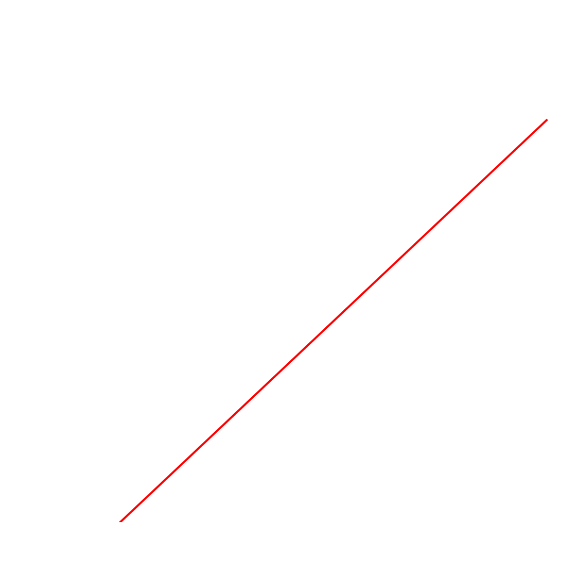
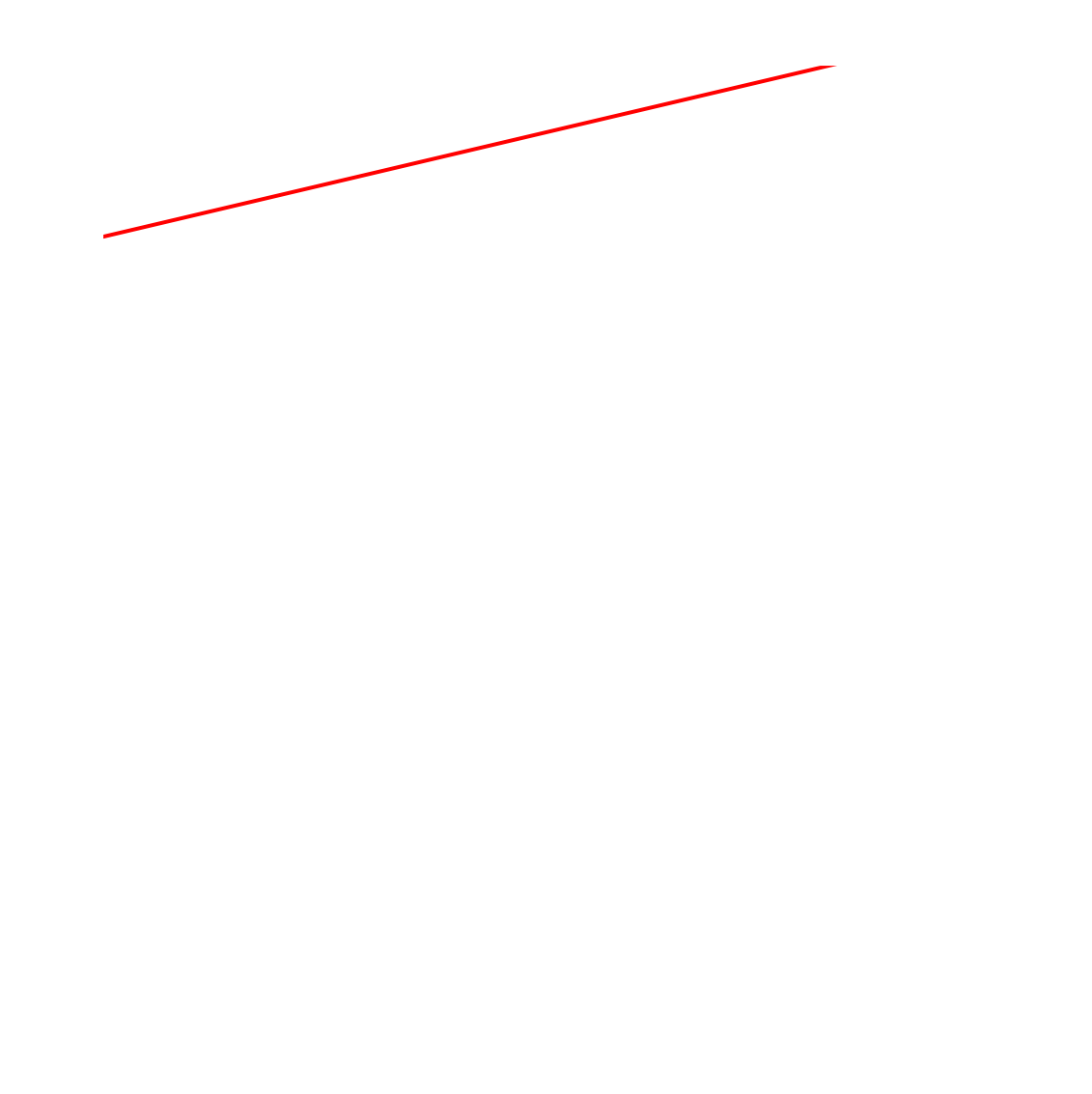
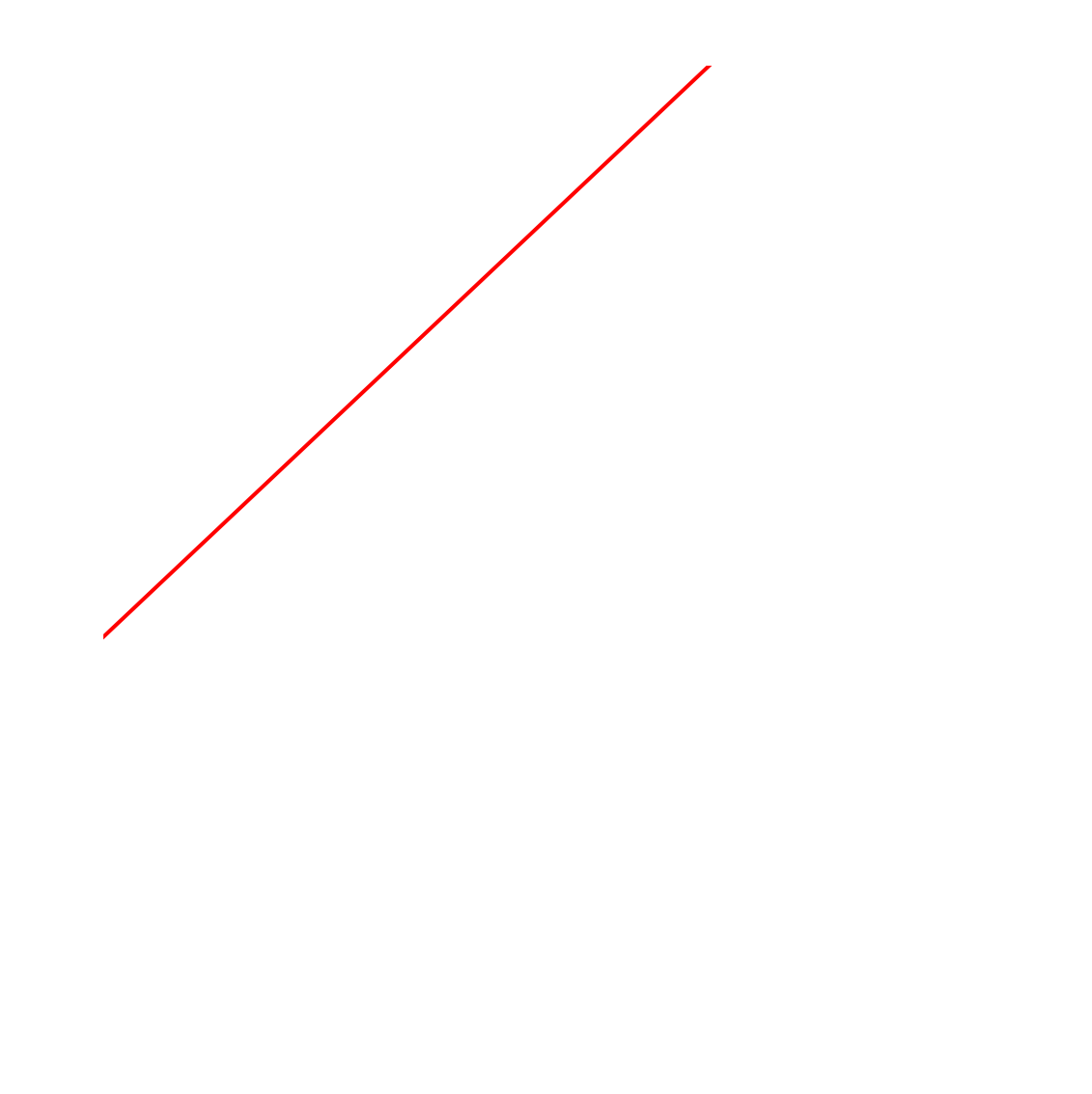
It seems an awful lot like you can do anything by stacking them.
Stacking isn’t too bad:
Multiplty, then
Check activations.
Fin
Source Code
---title: The XOR Problem---## Today- Thus far we have: - Created a matrix that can do a single intelligent task. - NOT general intelligence - Shown how to use random processes to create that matrix. - Not perfected this, by shown the ability to improve on random.# Motivation## Re-evaluating Our Model- We have been using a **single-layer** approach. - What does this mean? - We have a single "layer" of thinking neurons between the "sensory neurons" and result.```{dot}//| echo: falsegraph SudokuBipartite { rankdir=TB; bgcolor="transparent" node [shape=circle, fontcolor = "#ffffff", color = "#ffffff"] edge [color = "transparent"] // --- PARTITION 1: SRC --- subgraph cluster_cells { rankdir=LR; node [style=filled, fillcolor="red"]; C22 [label="(2,2)"]; C21 [label="(2,1)"]; C20 [label="(2,0)"]; C12 [label="(1,2)"]; C11 [label="(1,1)"]; C10 [label="(1,0)"]; C02 [label="(0,2)"]; C01 [label="(0,1)"]; C00 [label="(0,0)"]; } // --- PARTITION 2: DST --- subgraph cluster_cells { rankdir=RL; node [fillcolor="blue"]; D06 [label="6"]; D05 [label="5"]; D04 [label="4"]; D03 [label="3"]; D02 [label="2"]; D01 [label="1"]; } // ROW 0 C00 -- {D01 D02 D03 D04 D05 D06}; C01 -- {D01 D02 D03 D04 D05 D06}; C02 -- {D01 D02 D03 D04 D05 D06}; C10 -- {D01 D02 D03 D04 D05 D06}; C11 -- {D01 D02 D03 D04 D05 D06}; C12 -- {D01 D02 D03 D04 D05 D06}; C20 -- {D01 D02 D03 D04 D05 D06}; C21 -- {D01 D02 D03 D04 D05 D06}; C22 -- {D01 D02 D03 D04 D05 D06};}```## This... works- We have shown that there are possible matrix solutions that classify correctly in all cases using this single layer. - Given one (1) assumption.- Recall this solution:```{python}import numpy as npmulti = np.array([ [-1/1, -1/1, -1/1, -1/1, 1/1, -1/1, -1/1, -1/1, -1/1], [-1/2, -1/2, 1/2, -1/2, -1/2, -1/2, 1/2, -1/2, -1/2], [-1/3, -1/3, 1/3, -1/3, 1/3, -1/3, 1/3, -1/3, -1/3], [ 1/4, -1/4, 1/4, -1/4, -1/4, -1/4, 1/4, -1/4, 1/4], [ 1/5, -1/5, 1/5, -1/5, 1/5, -1/5, 1/5, -1/5, 1/5], [ 0/6, 3/6, 0/6, 3/6, -6/6, 3/6, 0/6, 3/6, 0/6],])```## Big Assumption- We made a big, I'd argue unreasonable, assumption.- Three must always look like this: - `[0,0,1,0,1,0,1,0,0]`- Never like this: - `[1,0,0,0,1,0,0,0,1]`## Encoding the Number 3:::: {.columns}::: {.column width="50%"}| | | ||:-:|:-:|:-:|| 0 | 0 | **1** || 0 | **1** | 0 || **1** | 0 | 0 |:::::: {.column width="50%"}<div style="position: relative; width: 300px; height: 300px; background-color: white; border: 1px solid #ccc;"><div style="position: absolute; top: 0; right: 0; width: 100px; height: 100px; background-color: black;"></div><div style="position: absolute; top: 50%; left: 50%; transform: translate(-50%, -50%); width: 100px; height: 100px; background-color: black;"></div><div style="position: absolute; bottom: 0; left: 0; width: 100px; height: 100px; background-color: black;"></div></div>:::::::## Why?- Is it not equally correct to have that die rotated 90°?- Is that not still a die showing a three?## Re-encoding the Number 3:::: {.columns}::: {.column width="50%"}| | | ||:-:|:-:|:-:|| **1** | 0 | 0 || 0 | **1** | 0 || 0 | 0 | **1** |:::::: {.column width="50%"}<div style="position: relative; width: 300px; height: 300px; background-color: white; border: 1px solid #ccc;"><div style="position: absolute; bottom: 0; right: 0; width: 100px; height: 100px; background-color: black;"></div><div style="position: absolute; top: 50%; left: 50%; transform: translate(-50%, -50%); width: 100px; height: 100px; background-color: black;"></div><div style="position: absolute; top: 0; left: 0; width: 100px; height: 100px; background-color: black;"></div></div>:::::::## Try it!- We can take a look at how well we classify this value.- First, we make both "top left" and "top right" three.```{python}rite = [0,0,1,0,1,0,1,0,0]left = [1,0,0,0,1,0,0,0,1]```# Aside: Matrix Review## Classify it!- As with anything else, we can take our trusty "multi-classifier".```{python}multi.shape```- As a $6 \times 9$ matrix, we can use it to take something of size "9" - like the 9 possible dots on a die - and get something of size 6 - like the six possible values of a die.## Matrix Multiply- To perform a multiplication, we take our die and multiply it by each internal sub-vector of size 9 of the matrix. - Make sure you understand that sentence.## I could...- It is possible to just take a each row, multiply by the die, and see the result.```{python}for row in multi:print(rite * row)```## I could...- We could then sum up each row...```{python}for row in multi:print(sum(rite * row))```## I could...- We could then compare the sum to `1````{python}for row in multi:print(1<=sum(rite * row))```## Transpose- We do not have to use a `for` loop - This is a simple case of *matrix multiplication*- Matrix multiplication - Multiplies rows of the first matrix by the columns of the next. - Sums the rows. - Outputs the sum of the row in the relevant position in a vector.## Worked Example- Here is an example...- I hastily wrote `multi` as a $6 \times 9$...```{python}multi```- So the *rows* are of length 9.## Transpose- ...so I need to rotate (transpose) it.- So the *columns* are of length 9.```{python}multi.transpose()```- Transpose has a `()` at the end because it is an action (a *verb*)## Multiply- Then, I can use `@` to "matrix multiply" the dice times the classifier!```{python}rite @ multi.transpose()```## The Bias- To determine if this is enough for a neuron to fire, I still need to include the bias. - This isn't part of matrix multiplication!- So we do so, same as with the other method using `sum` and `for````{python}1<= rite @ multi.transpose()```## The problem- This classifier only works for the "top right" version of three!```{python}1<= left @ multi.transpose()```- Even though that is definitely a three!```{python}sum(left)```# Interactions## Our method...- ... works well for detecting a **single dot**.- But what happens when dots **interact**?- We encounter a limit of our current logic.## Two vs. Four- Let's look at the **two** and **four** dice.- Both have dots in *either* the **top-left** *or* **top-right**.- The four simply has dots in *both* the **top-left** *and* **bottom-right**.:::: {.columns}::: {.column width="33%"}<div style="position: relative; width: 300px; height: 300px; background-color: white; border: 1px solid #ccc;"><div style="position: absolute; top: 0; right: 0; width: 100px; height: 100px; background-color: black;"></div><div style="position: absolute; bottom: 0; left: 0; width: 100px; height: 100px; background-color: black;"></div></div>:::::: {.column width="34%"}<div style="position: relative; width: 300px; height: 300px; background-color: white; border: 1px solid #ccc;"><div style="position: absolute; bottom: 0; right: 0; width: 100px; height: 100px; background-color: black;"></div><div style="position: absolute; top: 0; left: 0; width: 100px; height: 100px; background-color: black;"></div></div>:::::: {.column width="33%"}<div style="position: relative; width: 300px; height: 300px; background-color: white; border: 1px solid #ccc;"><div style="position: absolute; bottom: 0; right: 0; width: 100px; height: 100px; background-color: black;"></div><div style="position: absolute; top: 0; right: 0; width: 100px; height: 100px; background-color: black;"></div><div style="position: absolute; bottom: 0; left: 0; width: 100px; height: 100px; background-color: black;"></div><div style="position: absolute; top: 0; left: 0; width: 100px; height: 100px; background-color: black;"></div></div>:::::::## Three vs. Five- Both have a **center dot** and a diagonal.- Both have dots in *either* the **top-left** *or* **top-right**.- The five simply has dots in *both* the **top-left** *and* **bottom-right**.:::: {.columns}::: {.column width="33%"}<div style="position: relative; width: 300px; height: 300px; background-color: white; border: 1px solid #ccc;"><div style="position: absolute; top: 0; right: 0; width: 100px; height: 100px; background-color: black;"></div><div style="position: absolute; top: 50%; left: 50%; transform: translate(-50%, -50%); width: 100px; height: 100px; background-color: black;"></div><div style="position: absolute; bottom: 0; left: 0; width: 100px; height: 100px; background-color: black;"></div></div>:::::: {.column width="34%"}<div style="position: relative; width: 300px; height: 300px; background-color: white; border: 1px solid #ccc;"><div style="position: absolute; bottom: 0; right: 0; width: 100px; height: 100px; background-color: black;"></div><div style="position: absolute; top: 50%; left: 50%; transform: translate(-50%, -50%); width: 100px; height: 100px; background-color: black;"></div><div style="position: absolute; top: 0; left: 0; width: 100px; height: 100px; background-color: black;"></div></div>:::::: {.column width="33%"}<div style="position: relative; width: 300px; height: 300px; background-color: white; border: 1px solid #ccc;"><div style="position: absolute; bottom: 0; right: 0; width: 100px; height: 100px; background-color: black;"></div><div style="position: absolute; top: 0; right: 0; width: 100px; height: 100px; background-color: black;"></div><div style="position: absolute; bottom: 0; left: 0; width: 100px; height: 100px; background-color: black;"></div><div style="position: absolute; top: 50%; left: 50%; transform: translate(-50%, -50%); width: 100px; height: 100px; background-color: black;"></div><div style="position: absolute; top: 0; left: 0; width: 100px; height: 100px; background-color: black;"></div></div>:::::::## The Interaction Problem- Our matrix multiplication is a **linear combination**.- It sums up evidence: $y = \sum w_i x_i$.- To tell a 2 from a 4, we need more than a sum. - 4 will **always** sum more than 2, *unless we restrict 2 to a single orientation*- We need to know if dots exist **exclusively**.## A Minimal Example- Let's focus on just **two positions** on the die.- Position A: Top-Left dot ($x_1$).- Position B: Top-Right dot ($x_2$).- Can we "calculate" a specific relationship?## The Four Scenarios- We take $(x_1, x_2)$ to be... - Scenario 1: No dots are present (0, 0). - Scenario 2: Only Top-Left is present (1, 0). - Scenario 3: Only Top-Right is present (0, 1). - Scenario 4: Both dots are present (1, 1).## Defining XOR- **XOR** stands for **Exclusive OR**.- Pronounced as "ex-or" or "ZOR".- It means: "Either A or B, but **not both**."- It is a fundamental technique in logic and computing. - Not so much the English language! - English tends to use "or" for "xor" and nothing for "logical or", which is either of "and" and "xor".## XOR vs. OR- In a standard (logical) **OR**, (1, 1) results in True. - Not "coke or pepsi" (restaurant only has one) - Perhaps "delicious or filling" (wouldn't reject a dish that is *both*)- In an **XOR**, (1, 1) results in **False**. - Perhaps, when ordering sides, "fries or tots" - Both would cost extra and is therefore banned.- This "reversal" is what breaks simple models.## XOR in Real Life- **Dairy Choice**: Choose milk or soy, but not both.- **Enrollment**: You can "Enroll" or "Drop," not both.- **Car "Status"**: Engine is either running or "off"- Logic depends on specific, exclusive combinations.## Coding the Problem- Let's try to build an XOR dataset in NumPy.- We want to see if our perceptron can solve it. - We want to regard this as only trying to tell "small" (2 or 3) from "big" (4 or 5) numbers by looking at the top outer two dots.- The "x" in XOR stands for "exclusive or"- I use "i" for "inclusive or" to not just say vanilla "or"```{python}x = np.array([[0,0], [0,1], [1,0], [1,1]])y_xor = np.array([0, 1, 1, 0])y_ior = np.array([0, 1, 1, 1])```# Linearity## The Geometry of Logic- Imagine a 2D plot of these points.- X-axis: Top-Left dot ($x_1$).- Y-axis: Top-Right dot ($x_2$).- Let's visualize the "IOR" logic first.## Meaning- We want to place a line somewhere through this 2D space. - On one side of the line, the neuron "activates". - On the other, it does not.- IOR is relatively simple (the 4/5 case) - we only want to activate if we see both dots.## Place dots```{python}#| echo: falseimport matplotlib.pyplot as plt# Points and their labelspoints = [(1, 0), (0, 1), (1, 1), (0, 0)]labels = ["top right only", "top left only", "both top", "none"]x_coords = [p[0] for p in points]y_coords = [p[1] for p in points]# Set the figure to be transparentfig, ax = plt.figure(figsize=(6, 6), facecolor='none'), plt.gca()# Set axes background to transparentax.set_facecolor('none')# Plot the points (all white dots)ax.scatter(x_coords, y_coords, color='white', s=150) # Increased size for better visibility on dark backgrounds# Annotate each point (all white text)for i, label inenumerate(labels): ax.annotate(label, (x_coords[i], y_coords[i]), textcoords="offset points", xytext=(0, 15), ha='center', fontsize=12, fontweight='bold', color='white')# Set labels (all white text)ax.set_xlabel("Top Right Dot (x1)", fontsize=14, color='white')ax.set_ylabel("Top Left Dot (x2)", fontsize=14, color='white')ax.set_title("The XOR Problem Geometry", fontsize=16, color='white')# Remove the gridax.grid(False)# Set axes to only show integer points 0 and 1 (white ticks)ax.set_xticks([0, 1])ax.set_yticks([0, 1])ax.tick_params(axis='both', colors='white', labelsize=12)# Set axis spine colors (white axes)ax.spines['bottom'].set_color('white')ax.spines['top'].set_color('white')ax.spines['left'].set_color('white')ax.spines['right'].set_color('white')# Adjust limits to see the points clearly without too much dead spaceax.set_xlim(-0.5, 1.5)ax.set_ylim(-0.5, 1.5)# Ensure the axes cross at a reasonable point or are clearly visible (white lines)ax.axhline(0, color='white', linewidth=1)ax.axvline(0, color='white', linewidth=1)# Set the overall plot color scheme to dark for contrast when displayed, but the save itself is transparent# For the sake of the user's current environment, we'll save with a transparent background.plt.tight_layout()```## Draw some lines- Any upward line either: - Doesn't capture all 2s or 3s, or - Captures all 2s or 3s but also captures all 4s or 5s - It can be wrong in both ways at once!- Some examples## Missing some 2s/3s```{python}#| echo: falseimport matplotlib.pyplot as pltimport numpy as np# Points and their labelspoints = [(1, 0), (0, 1), (1, 1), (0, 0)]labels = ["top right only", "top left only", "both top", "none"]x_coords = [p[0] for p in points]y_coords = [p[1] for p in points]# Set the figure to be transparentfig, ax = plt.figure(figsize=(6, 6), facecolor='none'), plt.gca()# Set axes background to transparentax.set_facecolor('none')# Plot the points (all white dots)ax.scatter(x_coords, y_coords, color='white', s=150) # Increased size for better visibility on dark backgrounds# Annotate each point (all white text)for i, label inenumerate(labels): ax.annotate(label, (x_coords[i], y_coords[i]), textcoords="offset points", xytext=(0, 15), ha='center', fontsize=12, fontweight='bold', color='white')# Set labels (all white text)ax.set_xlabel("Top Right Dot (x1)", fontsize=14, color='white')ax.set_ylabel("Top Left Dot (x2)", fontsize=14, color='white')ax.set_title("The XOR Problem Geometry", fontsize=16, color='white')# Remove the gridax.grid(False)# Set axes to only show integer points 0 and 1 (white ticks)ax.set_xticks([0, 1])ax.set_yticks([0, 1])ax.tick_params(axis='both', colors='white', labelsize=12)# Set axis spine colors (white axes)ax.spines['bottom'].set_color('white')ax.spines['top'].set_color('white')ax.spines['left'].set_color('white')ax.spines['right'].set_color('white')# Adjust limits to see the points clearly without too much dead spaceax.set_xlim(-0.5, 1.5)ax.set_ylim(-0.5, 1.5)# Ensure the axes cross at a reasonable point or are clearly visible (white lines)ax.axhline(0, color='white', linewidth=1)ax.axvline(0, color='white', linewidth=1)xs = np.arange(-5,15) /10ys = xs -.25plt.plot(xs, ys, "r")plt.tight_layout()```## Getting the 4s/5s```{python}#| echo: falseimport matplotlib.pyplot as pltimport numpy as np# Points and their labelspoints = [(1, 0), (0, 1), (1, 1), (0, 0)]labels = ["top right only", "top left only", "both top", "none"]x_coords = [p[0] for p in points]y_coords = [p[1] for p in points]# Set the figure to be transparentfig, ax = plt.figure(figsize=(6, 6), facecolor='none'), plt.gca()# Set axes background to transparentax.set_facecolor('none')# Plot the points (all white dots)ax.scatter(x_coords, y_coords, color='white', s=150) # Increased size for better visibility on dark backgrounds# Annotate each point (all white text)for i, label inenumerate(labels): ax.annotate(label, (x_coords[i], y_coords[i]), textcoords="offset points", xytext=(0, 15), ha='center', fontsize=12, fontweight='bold', color='white')# Set labels (all white text)ax.set_xlabel("Top Right Dot (x1)", fontsize=14, color='white')ax.set_ylabel("Top Left Dot (x2)", fontsize=14, color='white')ax.set_title("The XOR Problem Geometry", fontsize=16, color='white')# Remove the gridax.grid(False)# Set axes to only show integer points 0 and 1 (white ticks)ax.set_xticks([0, 1])ax.set_yticks([0, 1])ax.tick_params(axis='both', colors='white', labelsize=12)# Set axis spine colors (white axes)ax.spines['bottom'].set_color('white')ax.spines['top'].set_color('white')ax.spines['left'].set_color('white')ax.spines['right'].set_color('white')# Adjust limits to see the points clearly without too much dead spaceax.set_xlim(-0.5, 1.5)ax.set_ylim(-0.5, 1.5)# Ensure the axes cross at a reasonable point or are clearly visible (white lines)ax.axhline(0, color='white', linewidth=1)ax.axvline(0, color='white', linewidth=1)xs = np.arange(-5,15) /10ys = xs/4+1.25plt.plot(xs, ys, "r")plt.tight_layout()```## Both Bad Things ```{python}#| echo: falseimport matplotlib.pyplot as pltimport numpy as np# Points and their labelspoints = [(1, 0), (0, 1), (1, 1), (0, 0)]labels = ["top right only", "top left only", "both top", "none"]x_coords = [p[0] for p in points]y_coords = [p[1] for p in points]# Set the figure to be transparentfig, ax = plt.figure(figsize=(6, 6), facecolor='none'), plt.gca()# Set axes background to transparentax.set_facecolor('none')# Plot the points (all white dots)ax.scatter(x_coords, y_coords, color='white', s=150) # Increased size for better visibility on dark backgrounds# Annotate each point (all white text)for i, label inenumerate(labels): ax.annotate(label, (x_coords[i], y_coords[i]), textcoords="offset points", xytext=(0, 15), ha='center', fontsize=12, fontweight='bold', color='white')# Set labels (all white text)ax.set_xlabel("Top Right Dot (x1)", fontsize=14, color='white')ax.set_ylabel("Top Left Dot (x2)", fontsize=14, color='white')ax.set_title("The XOR Problem Geometry", fontsize=16, color='white')# Remove the gridax.grid(False)# Set axes to only show integer points 0 and 1 (white ticks)ax.set_xticks([0, 1])ax.set_yticks([0, 1])ax.tick_params(axis='both', colors='white', labelsize=12)# Set axis spine colors (white axes)ax.spines['bottom'].set_color('white')ax.spines['top'].set_color('white')ax.spines['left'].set_color('white')ax.spines['right'].set_color('white')# Adjust limits to see the points clearly without too much dead spaceax.set_xlim(-0.5, 1.5)ax.set_ylim(-0.5, 1.5)# Ensure the axes cross at a reasonable point or are clearly visible (white lines)ax.axhline(0, color='white', linewidth=1)ax.axvline(0, color='white', linewidth=1)xs = np.arange(-5,15) /10ys = xs +.75plt.plot(xs, ys, "r")plt.tight_layout()```## Takeaway- This is no possible way for a **single-layer** perceptron to differentiate 2s/3s from 4s/5s.- On these graphs, the "intercept" represents the bias.- On these graphs, the "slope" represents (the sume of) the weights## Impact on Dice- To distinguish a 2 from a 4 based on these dots:- We need to know if the extra dots are **absent**.- Our current model only knows how to **add weight**.- It doesn't know how to handle "exclusive" patterns.## Linear Combinations- Our current math looks like this:- $Output = Weights \cdot Inputs + Bias$- This is a **linear** transformation.- It can only create "flat" decision boundaries.# Layers## The Solution?- To solve XOR, we need a *more powerful technique*- We will: - Create something not unlike a perceptron which "projects" these two dots into a different "space" - Apply that transformation to the incoming (visual) data. - Apply a perceptron to the transformed data.- These are two perceptron "layers"## Visualizing Layers- Think of the first layer as "feature detectors."- One neuron detects "At least one dot."- Another neuron detects "Both dots."- The final layer combines these detections.## Designing the Logic- XOR can be thought of as:- (A IOR B) **AND NOT** (A AND B).- This requires a sequence of operations.- Sequence = **Depth** in a neural network.## Minimal Example- We consider only "corners in the top row".- These ones in red, basically:<div style="position: relative; width: 300px; height: 300px; background-color: white; border: 1px solid #ccc;"><div style="position: absolute; top: 0; right: 0; width: 100px; height: 100px; background-color: red;"></div><div style="position: absolute; top: 0; left: 0; width: 100px; height: 100px; background-color: red;"></div></div>- We will make a "perceptron" that takes only two inputs.## Data- We recall:```{python}print(x)``````{python}print(y_ior)``````{python}print(y_xor)```- We want to take a vector of size 2 (top two dots) and produce a vecotr of size 2 (IOR or XOR). - Only XOR is interesting.## Our First Steps:::: {.columns}::: {.column width="50%"}- First, let's naively just sum up the number of dots.- We can do this simply with a single layer that sets all weights to 1.:::::: {.column width="50%"}```{dot}//| echo: false//| fig-width: 400pxgraph SudokuBipartite { rankdir=TB; bgcolor="transparent" node [shape=circle, fontcolor = "#ffffff", color = "#ffffff"] edge [color = "white"] // --- PARTITION 1: SRC --- subgraph cluster_cells { rankdir=LR; node [style=filled, fillcolor="magenta"]; RITE [label="Top Rite"]; LEFT [label="Top Left"]; } // --- PARTITION 2: DST --- subgraph cluster_cells { rankdir=RL; node [fillcolor="blue"]; DEST [label="Neuron"] } RITE -- DEST; LEFT -- DEST;}```:::::::## Our First Steps:::: {.columns}::: {.column width="50%"}- We can have neurons fire for sums of *at least* 1 or *at least* 2.- Green for "positive" weights (greater than zero):::::: {.column width="50%"}```{dot}//| echo: false//| fig-width: 400pxgraph SudokuBipartite { rankdir=TB; bgcolor="transparent" node [shape=circle, fontcolor = "#ffffff", color = "#ffffff"] edge [color = "green"] // --- PARTITION 1: SRC --- subgraph cluster_cells { rankdir=LR; node [style=filled, fillcolor="magenta"]; RITE [label="Top Rite"]; LEFT [label="Top Left"]; } // --- PARTITION 2: DST --- subgraph cluster_cells { rankdir=RL; node [fillcolor="blue"]; ONE [label="1"]; TWO [label="2"]; } {RITE, LEFT} -- ONE; {RITE, LEFT} -- TWO;}```:::::::## Setting Weights:::: {.columns}::: {.column width="50%"}- Apply high weight to edges into `1`- Apply half weight to edges into `2`:::::: {.column width="50%"}```{dot}//| echo: false//| fig-width: 400pxgraph SudokuBipartite { rankdir=TB; bgcolor="transparent" node [shape=circle, fontcolor = "#ffffff", color = "#ffffff"] edge [color = "green"] // --- PARTITION 1: SRC --- subgraph cluster_cells { rankdir=LR; node [style=filled, fillcolor="magenta"]; RITE [label="Top Rite"]; LEFT [label="Top Left"]; } // --- PARTITION 2: DST --- subgraph cluster_cells { rankdir=RL; node [fillcolor="blue"]; ONE [label="1"]; TWO [label="2"]; } {RITE, LEFT} -- ONE [penwidth=2.0]; {RITE, LEFT} -- TWO [penwidth=0.5];}```:::::::## Adding a Layer:::: {.columns}::: {.column width="50%"}- We keep this stage, but add a layer below.- We only connect top-to-middle and middle-to-bottom:::::: {.column width="50%"}```{dot}//| echo: false//| fig-width: 400pxgraph SudokuBipartite { rankdir=TB; bgcolor="transparent" node [shape=circle, fontcolor = "#ffffff", color = "#ffffff"] edge [color = "green"] // --- PARTITION 1: SRC --- subgraph cluster_cells { rankdir=LR; node [style=filled, fillcolor="magenta"]; RITE [label="Top Rite"]; LEFT [label="Top Left"]; } // --- PARTITION 2: DST --- subgraph cluster_cells { rankdir=RL; node [fillcolor="blue"]; ONE [label="1"]; TWO [label="2"]; } subgraph out_cells { rankdir=RL; node [fillcolor="orange"]; IOR; XOR; } {RITE, LEFT} -- ONE [penwidth=2.0]; {RITE, LEFT} -- TWO [penwidth=0.5]; ONE -- {IOR, XOR}; TWO -- {IOR, XOR};}```:::::::## Setting weights again :::: {.columns}::: {.column width="50%"}- We add a negative (red) weight from "2" to "XOR" - We don't want to "activate" if both are set:::::: {.column width="50%"}```{dot}//| echo: false//| fig-width: 400pxgraph SudokuBipartite { rankdir=TB; bgcolor="transparent" node [shape=circle, fontcolor = "#ffffff", color = "#ffffff"] edge [color = "green"] // --- PARTITION 1: SRC --- subgraph cluster_cells { rankdir=LR; node [style=filled, fillcolor="magenta"]; RITE [label="Top Rite"]; LEFT [label="Top Left"]; } // --- PARTITION 2: DST --- subgraph cluster_cells { rankdir=RL; node [fillcolor="blue"]; ONE [label="1"]; TWO [label="2"]; } subgraph out_cells { rankdir=RL; node [fillcolor="orange"]; IOR; XOR; } {RITE, LEFT} -- ONE [penwidth=2.0]; {RITE, LEFT} -- TWO [penwidth=0.5]; ONE -- {IOR, XOR}; TWO -- IOR; TWO -- XOR [color = "red"];}```:::::::## As a matrix- We can easily make a matrix!- ... or two.```{python}top_layer = np.array([ [ 1.0, 1.0], [ 0.5, 0.5],])``````{python}bot_layer = np.array([ [ 1.0, 1.0], [ 1.0, -1.0],])```## Try it- We can apply the first layer.```{python}np.array([0,1]) @ top_layer```## Transpose- Whoops! We have to transponse to use `@````{python}np.array([0,1]) @ top_layer.transpose()```## Activate- We can compare to `1` (or some other bias) to determine activation.```{python}1<= np.array([0,1]) @ top_layer.transpose()```## Next Layer- We can then multiply this *intermediate result* `int` by the next layer.```{python}(1<= np.array([0,1]) @ top_layer.transpose()) @ bot_layer.transpose()```## Activate Again- And we can compare that to activation. ```{python}1<= (1<= np.array([0,1]) @ top_layer.transpose()) @ bot_layer.transpose()```- Is this what we would expect? - Yes! - There is *exactly* one dot. - There is *at least* one dot.## Test 'em all- Check this out:```{python}for pair in x:print(pair, 1<= (1<= np.array(pair) @ top_layer.transpose()) @ bot_layer.transpose())```- *We can tell 2s/3s (middle) from 4s/5s (bottom)!*# Summary## What we learned- You can't do everything with a single matrix.- It seems an awful lot like you can do *anything* by stacking them.- Stacking isn't too bad: - Multiplty, then - Check activations.# Fin