graph Hiawatha {
    rankdir=TB;
    bgcolor="transparent"
    node [shape=circle, fontcolor = "#ffffff", color = "#ffffff"]
    edge [color = "#ffffff"]

    MKE -- MKA -- SVT -- GLN -- CHI
}Neural Networks
AI 101
Today
- Follow up on the adjacency matrix lab
- I will live-code this then post my solution on the website and link it here.
- Bipartite graphs
- Neurons
- Our first neural network
- (Single layer, fully-connected)
Matrix
- We recall matrices from the Sudoku lab.
The Adjacency Matrix
\[ \begin{bmatrix}1 & 9 & -13 \\20 & 5 & -6 \end{bmatrix} \]
Indices
- Mini-Sudoku is 4$$4.
- General, matrices may be \(m\) by \(n\).
\[ \mathbf{A} = \begin{pmatrix} a_{11} & a_{12} & \cdots & a_{1n} \\ a_{21} & a_{22} & \cdots & a_{2n} \\ \vdots & \vdots & \ddots & \vdots \\ a_{m1} & a_{m2} & \cdots & a_{mn} \\ \end{pmatrix} \]
Indices
- There are \(4 \times 4 = 16\) total “positions” in a Mini-Sudoku
- Each of these 16 “positions” are either impacted or non-impacted
- Each position is impacted by:
- Other positions in the same row.
- Other positions in the same column.
- Other positions in the same \(2\times2\) submatrix
- Each position is impacted by:
Encoding
- Vs. refer to each as, e.g. \(a_{mn}\).
- Just give each “position” a unique number:
Tedious
| \(a_{1,1}\) | \(a_{1,2}\) | \(a_{1,3}\) | \(a_{1,4}\) |
| \(a_{2,1}\) | \(a_{2,2}\) | \(a_{2,3}\) | \(a_{2,4}\) |
| \(a_{3,1}\) | \(a_{3,2}\) | \(a_{3,3}\) | \(a_{3,4}\) |
| \(a_{4,1}\) | \(a_{4,2}\) | \(a_{4,3}\) | \(a_{4,4}\) |
Brief
| 1 | 2 | 3 | 4 |
| 5 | 6 | 7 | 8 |
| 9 | 10 | 11 | 12 |
| 13 | 14 | 15 | 16 |
Example
- Consider the top left position.
| 1 | 2 | 3 | 4 |
| 5 | 6 | 7 | 8 |
| 9 | 10 | 11 | 12 |
| 13 | 14 | 15 | 16 |
Order
- We can write these down in numerical order.
| 1 | 2 | 3 | 4 | 5 | 6 | 7 | 8 | 9 | 10 | 11 | 12 | 13 | 14 | 15 | 16 |
|---|---|---|---|---|---|---|---|---|---|---|---|---|---|---|---|
Correspondence
- They correspond to the following matrix positions
| 1 | 2 | 3 | 4 | 5 | 6 | 7 | 8 | 9 | 10 | 11 | 12 | 13 | 14 | 15 | 16 |
|---|---|---|---|---|---|---|---|---|---|---|---|---|---|---|---|
| \(a_{1,1}\) | \(a_{1,2}\) | \(a_{1,3}\) | \(a_{1,4}\) | \(a_{2,1}\) | \(a_{2,2}\) | \(a_{2,3}\) | \(a_{2,4}\) | \(a_{3,1}\) | \(a_{3,2}\) | \(a_{3,3}\) | \(a_{3,4}\) | \(a_{4,1}\) | \(a_{4,2}\) | \(a_{4,3}\) | \(a_{4,4}\) |
1’s
- We can mark adjacent positions as one (
1)- Like this.
| 1 | 2 | 3 | 4 | 5 | 6 | 7 | 8 | 9 | 10 | 11 | 12 | 13 | 14 | 15 | 16 |
|---|---|---|---|---|---|---|---|---|---|---|---|---|---|---|---|
| 1 | 1 | 1 | 1 | 1 | 1 | 1 | 1 |
0’s
- We can mark adjacent positions as one (
1)- And others as zero.
| 1 | 2 | 3 | 4 | 5 | 6 | 7 | 8 | 9 | 10 | 11 | 12 | 13 | 14 | 15 | 16 |
|---|---|---|---|---|---|---|---|---|---|---|---|---|---|---|---|
| 1 | 1 | 1 | 1 | 1 | 1 | 0 | 0 | 1 | 0 | 0 | 0 | 1 | 0 | 0 | 0 |
Code Cells
- We can take that last row and treat it as list.
- Lists begin and end with boxy brackets
[] - Lists contain multiple values, like
0or1 - The values are separated by commas
,
- Lists begin and end with boxy brackets
- Was:
| 1 | 2 | 3 | 4 | 5 | 6 | 7 | 8 | 9 | 10 | 11 | 12 | 13 | 14 | 15 | 16 |
|---|---|---|---|---|---|---|---|---|---|---|---|---|---|---|---|
| 1 | 1 | 1 | 1 | 1 | 1 | 0 | 0 | 1 | 0 | 0 | 0 | 1 | 0 | 0 | 0 |
Further
- This corresponds to things adjancent to position “1”
- Next, we can do things adjacent to position “2”.
- Same submatrix, same row, different column.
Definition
- We can combine each list into a list of lists
- And so on.
Types of Graphs
A Type of Graph
- We have seen a few types of graphs.
- Amtrak
- Dichotomous key
- River valley
- Sudoku
Amtrak
- Amtrak routes. (Linear graph)
Decision Tree
- The decision tree. (Tree graph)
digraph OakKey {
    bgcolor="transparent"
    node [shape=box,  fontcolor="white", color="white"];
    edge [color="white", fontcolor="white"];

    // Questions/Nodes
    Start [label="Leaves are smooth with no teeth or lobes?"];
    Evergreen [label="Laves evergreen?"];
    GrowthHabit [label="Large Tree (not shrub)?"];
    LeafShape [label="Leaves more than 3x long as wide"];
    Bristles [label="Lobes/teeth bristle-tipped?"];
    LobeCount6 [label="3 or fewer lobes?"];
    LobeCount7 [label="9 or fewer lobes?"];

    // Species (Leaf nodes)
    LiveOak [label="Southern live oak"];
    DwarfOak [label="Dwarf live oak"];
    WillowOak [label="Willow oak"];
    ShingleOak [label="Shingle oak"];
    BlackjackOak [label="Blackjack oak"];
    RedOak [label="Northern red oak"];
    WhiteOak [label="White oak"];
    SwampOak [label="Swamp chestnut oak"];

    // Relationships
    Start -> Evergreen [label="True"];
    Start -> Bristles [label="False"];

    Evergreen -> GrowthHabit [label="True"];
    Evergreen -> LeafShape [label="False"];

    GrowthHabit -> LiveOak [label="True"];
    GrowthHabit -> DwarfOak [label="False"];

    LeafShape -> WillowOak [label="True"];
    LeafShape -> ShingleOak [label="False"];

    Bristles -> LobeCount6 [label="True"];
    Bristles -> LobeCount7 [label="False"];

    LobeCount6 -> BlackjackOak [label="True"];
    LobeCount6 -> RedOak [label="False"];

    LobeCount7 -> WhiteOak [label="True"];
    LobeCount7 -> SwampOak [label="False"];
}Rivers
- We’ll do rivers as edges. (Tree graph)
graph Gorge {
    rankdir=RL;
    bgcolor="transparent"
    node [shape=circle, fontcolor = "#ffffff", color = "#ffffff"]
    edge [fontcolor = "#ffffff", color = "#ffffff"]

    Richland -- "The Dalles" [label="Columbia", color="blue"]
    "The Dalles" -- Portland [label="Columbia", color="blue"]
    Portland -- Astoria [label="Columbia", color="blue"]
    Bend -- "The Dalles" [label="Deschutes", color="red"]
    Salem -- Portland [label="Willamette", color="green"]
}Mini-Sudoku (One)
- Just the top-left’s connections.
graph SudokuBipartite {
    rankdir=TB;
    bgcolor="transparent"
    node [shape=circle, fontcolor = "#ffffff", color = "#ffffff"]
    edge [color = "transparent"]


    // --- PARTITION 1: SRC ---
    subgraph cluster_cells {
        rankdir=LR;
        node [style=filled, fillcolor="red"];
        C33 [label="(3,3)"]; C32 [label="(3,2)"]; C31 [label="(3,1)"]; C30 [label="(3,0)"];
        C23 [label="(2,3)"]; C22 [label="(2,2)"]; C21 [label="(2,1)"]; C20 [label="(2,0)"];
        C13 [label="(1,3)"]; C12 [label="(1,2)"]; C11 [label="(1,1)"]; C10 [label="(1,0)"];
        C03 [label="(0,3)"]; C02 [label="(0,2)"]; C01 [label="(0,1)"]; C00 [label="(0,0)"];
    }

    // --- PARTITION 2: DST ---

    subgraph cluster_cells {
        rankdir=RL;
        node [fillcolor="blue"];
        // Defining 16 cells (row, column)
        D33 [label="(3,3)"]; D32 [label="(3,2)"]; D31 [label="(3,1)"]; D30 [label="(3,0)"];
        D23 [label="(2,3)"]; D22 [label="(2,2)"]; D21 [label="(2,1)"]; D20 [label="(2,0)"];
        D13 [label="(1,3)"]; D12 [label="(1,2)"]; D11 [label="(1,1)"]; D10 [label="(1,0)"];
        D03 [label="(0,3)"]; D02 [label="(0,2)"]; D01 [label="(0,1)"]; D00 [label="(0,0)"];
    }

    // ROW 0
    C00 -- {D00 D01 D02 D03 D10 D20 D30 D11} [color = "#ffffff"];
    C01 -- {D00 D01 D02 D03 D11 D21 D31 D10};
    C02 -- {D00 D01 D02 D03 D12 D22 D32 D13};
    C03 -- {D00 D01 D02 D03 D13 D23 D33 D12};

    // ROW 1
    C10 -- {D10 D11 D12 D13 D00 D20 D30 D01};
    C11 -- {D10 D11 D12 D13 D01 D21 D31 D00};
    C12 -- {D10 D11 D12 D13 D02 D22 D32 D03};
    C13 -- {D10 D11 D12 D13 D03 D23 D33 D02};

    // ROW 2
    C20 -- {D20 D21 D22 D23 D00 D10 D30 D31};
    C21 -- {D20 D21 D22 D23 D01 D11 D31 D30};
    C22 -- {D20 D21 D22 D23 D02 D12 D32 D33};
    C23 -- {D20 D21 D22 D23 D03 D13 D33 D32};

    // ROW 3
    C30 -- {D30 D31 D32 D33 D00 D10 D20 D21};
    C31 -- {D30 D31 D32 D33 D01 D11 D21 D20};
    C32 -- {D30 D31 D32 D33 D02 D12 D22 D23};
    C33 -- {D30 D31 D32 D33 D03 D13 D23 D22};
}Mini-Sudoku (All)
- All connections
graph SudokuBipartite {
    rankdir=TD;
    bgcolor="transparent"
    node [shape=circle, fontcolor = "#ffffff", color = "#ffffff"]
    edge [color = "#ffffff"]


    // --- PARTITION 1: SRC ---
    subgraph cluster_cells {
        rankdir=LR;
        node [style=filled, fillcolor="red"];
        C33 [label="(3,3)"]; C32 [label="(3,2)"]; C31 [label="(3,1)"]; C30 [label="(3,0)"];
        C23 [label="(2,3)"]; C22 [label="(2,2)"]; C21 [label="(2,1)"]; C20 [label="(2,0)"];
        C13 [label="(1,3)"]; C12 [label="(1,2)"]; C11 [label="(1,1)"]; C10 [label="(1,0)"];
        C03 [label="(0,3)"]; C02 [label="(0,2)"]; C01 [label="(0,1)"]; C00 [label="(0,0)"];
    }

    // --- PARTITION 2: DST ---

    subgraph cluster_cells {
        rankdir=RL;
        node [fillcolor="blue"];
        // Defining 16 cells (row, column)
        D33 [label="(3,3)"]; D32 [label="(3,2)"]; D31 [label="(3,1)"]; D30 [label="(3,0)"];
        D23 [label="(2,3)"]; D22 [label="(2,2)"]; D21 [label="(2,1)"]; D20 [label="(2,0)"];
        D13 [label="(1,3)"]; D12 [label="(1,2)"]; D11 [label="(1,1)"]; D10 [label="(1,0)"];
        D03 [label="(0,3)"]; D02 [label="(0,2)"]; D01 [label="(0,1)"]; D00 [label="(0,0)"];
    }


    // ROW 0
    C00 -- {D00 D01 D02 D03 D10 D20 D30 D11};
    C01 -- {D00 D01 D02 D03 D11 D21 D31 D10};
    C02 -- {D00 D01 D02 D03 D12 D22 D32 D13};
    C03 -- {D00 D01 D02 D03 D13 D23 D33 D12};

    // ROW 1
    C10 -- {D10 D11 D12 D13 D00 D20 D30 D01};
    C11 -- {D10 D11 D12 D13 D01 D21 D31 D00};
    C12 -- {D10 D11 D12 D13 D02 D22 D32 D03};
    C13 -- {D10 D11 D12 D13 D03 D23 D33 D02};

    // ROW 2
    C20 -- {D20 D21 D22 D23 D00 D10 D30 D31};
    C21 -- {D20 D21 D22 D23 D01 D11 D31 D30};
    C22 -- {D20 D21 D22 D23 D02 D12 D32 D33};
    C23 -- {D20 D21 D22 D23 D03 D13 D33 D32};

    // ROW 3
    C30 -- {D30 D31 D32 D33 D00 D10 D20 D21};
    C31 -- {D30 D31 D32 D33 D01 D11 D21 D20};
    C32 -- {D30 D31 D32 D33 D02 D12 D22 D23};
    C33 -- {D30 D31 D32 D33 D03 D13 D23 D22};
}Bipartite
Definition
- The mini-sudoku graph is a bipartite graph
- Two collections of nodes.
- Every edge goes from one collection to the other.
- It just means two parts.
Examples
- Here’s a canonical representation from Wikipedia

Other Bipartite Graphs
- A common one is students-to-universities
graph SudokuBipartite {
    rankdir=TD;
    bgcolor="transparent"
    node [shape=circle, fontcolor = "#ffffff", color = "#ffffff"]
    edge [color = "#ffffff"]


    // --- PARTITION 1: SRC ---
    subgraph cluster_cells {
        rankdir=LR;
        node [style=filled, fillcolor="red"];
        C13 [label="Just Like Normal People"];
        C23 [label="Children of Professors"];
        C33 [label="Children of Presidents"];
    }

    // --- PARTITION 2: DST ---

    subgraph cluster_cells {
        rankdir=RL;
        node [fillcolor="blue"];
        // Defining 16 cells (row, column)
        D13 [label="Just Like College"];
        D23 [label="Highly Selective"];
        D33 [label="Ivy League Peers"];
    }

    C33 -- D33
    C23 -- D23
    C13 -- D13
}Other Bipartite Graphs
- Couples on The Breakfast Club (1985)
graph SudokuBipartite {
    rankdir=TD;
    bgcolor="transparent"
    node [shape=circle, fontcolor = "#ffffff", color = "#ffffff"]
    edge [color = "#ffffff"]

    // --- PARTITION 2: DST ---
    subgraph cluster_cells {
        node [style=filled, fillcolor="blue"];
        // Defining 16 cells (row, column)
        D13 [label="Claire (Princess)"];
        D23 [label="Allison (Basket Case)"];
    }

    // --- PARTITION 1: SRC ---
    subgraph cluster_cells {
        node [style=filled, fillcolor="red"];
        C13 [label="Andrew (Athlete)"];
        C23 [label="Brian (Brain)"];
        C33 [label="Bender (Criminal)"];
    }


    D13 -- C33
    D23 -- C13
    D13 -- C23 [color="transparent"]
    D23 -- C23 [color="transparent"]
}The Brain?
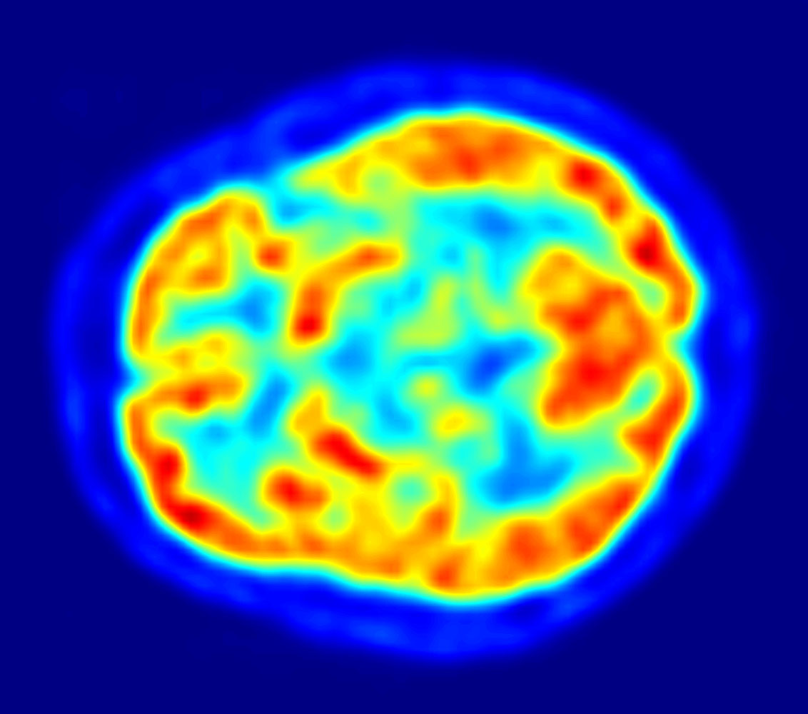
The Neuron
Neurons
- There are biological neurons.
- Brain cells
- Actually exist
- There are theoretical, machine learning or AI neurons
- Don’t “actually” exist
- Are simulated by computers
Image, UOregon
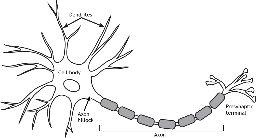
Neurons as Nodes
- We can treat each cell body as a node in a graph.
- Or train station in Amtrak.
- We can treat each axon as an edge in graph.
- Or train connection in Amtrak
Brains as Graphs
- Somehow, information reaches the brain.
- We’ll just not worry about that for now, but…
- Touch in the hands/skins
- Vision in the eye
- Olfaction, temperature, etc.
- We’ll call these sensory neurons
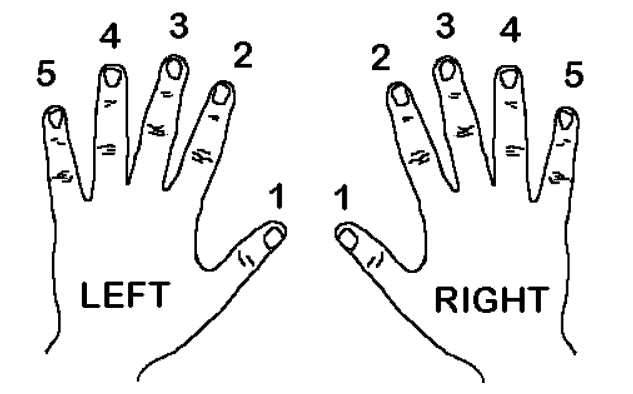
Example
- We imagine, for example, a sensory neuron in each finger.
- We’ll use a numbering from piano instruction.
graph SudokuBipartite {
    rankdir=TD;
    bgcolor="transparent"
    node [shape=circle, fontcolor = "#ffffff", color = "#ffffff"]
    edge [color = "#ffffff"]


    // --- PARTITION 1: SRC ---
    subgraph cluster_cells {
        rankdir=LR;
        node [style=filled, fillcolor="red"];
        R5 ; R4 ; R3 ; R2 ; R1 ; L1 ; L2 ; L3 ; L4 ; L5 ;
    }

}Regard
- Fingers as the top, sensing layer in RED
- Neurons in the brain as the lower, thinking layer in BLUE
graph SudokuBipartite {
    rankdir=TD;
    bgcolor="transparent"
    node [shape=circle, fontcolor = "#ffffff", color = "#ffffff"]
    edge [color = "transparent"]


    // --- PARTITION 1: SRC ---
    subgraph cluster_cells {
        rankdir=LR;
        node [style=filled, fillcolor="red"];
        R5 ; R4 ; R3 ; R2 ; R1 ; L1 ; L2 ; L3 ; L4 ; L5 ;
    }

    // --- PARTITION 2: DST ---
    subgraph cluster_cells {
        rankdir=LR;
        node [style=filled, fillcolor="blue"];
        B0 ; B9 ; B8 ; B7 ; B6 ; B5 ; B4 ; B3 ; B2 ; B1 ;
    }

    R5 -- B0 ;
    R4 -- B9 ;
    R3 -- B8 ;
    R2 -- B7 ;
    R1 -- B6 ;

    L1 -- B5 ;
    L2 -- B4 ;
    L3 -- B3 ;
    L4 -- B2 ;
    L5 -- B1 ;

}Meaning
- Perhaps the braincell “B3” encodes good movie
- I usually use give two thumbs up - both “R1” and “L1”.
graph SudokuBipartite {
    rankdir=TD;
    bgcolor="transparent"
    node [shape=circle, fontcolor = "#ffffff", color = "#ffffff"]
    edge [color = "transparent"]


    // --- PARTITION 1: SRC ---
    subgraph cluster_cells {
        rankdir=LR;
        node [style=filled, fillcolor="red"];
        R5 ; R4 ; R3 ; R2 ; R1 ; L1 ; L2 ; L3 ; L4 ; L5 ;
    }

    // --- PARTITION 2: DST ---
    subgraph cluster_cells {
        rankdir=LR;
        node [style=filled, fillcolor="blue"];
        B0 ; B9 ; B8 ; B7 ; B6 ; B5 ; B4 ; B3 ; B2 ; B1 ;
    }

    R5 -- B0 ;
    R4 -- B9 ;
    R3 -- B8 ;
    R2 -- B7 ;
    R1 -- B6 ;

    L1 -- B5 ;
    L2 -- B4 ;
    L3 -- B3 ;
    L4 -- B2 ;
    L5 -- B1 ;

    L1 -- B3 [color="#ffffff"] ;
    R1 -- B3 [color="#ffffff"] ;

}
Meaning
- Perhaps the braincell “B5” encodes “pinch of salt”
- I usually use right thumb and index finger - R1 and R2
graph SudokuBipartite {
    rankdir=TD;
    bgcolor="transparent"
    node [shape=circle, fontcolor = "#ffffff", color = "#ffffff"]
    edge [color = "transparent"]


    // --- PARTITION 1: SRC ---
    subgraph cluster_cells {
        rankdir=LR;
        node [style=filled, fillcolor="red"];
        R5 ; R4 ; R3 ; R2 ; R1 ; L1 ; L2 ; L3 ; L4 ; L5 ;
    }

    // --- PARTITION 2: DST ---
    subgraph cluster_cells {
        rankdir=LR;
        node [style=filled, fillcolor="blue"];
        B0 ; B9 ; B8 ; B7 ; B6 ; B5 ; B4 ; B3 ; B2 ; B1 ;
    }

    R5 -- B0 ;
    R4 -- B9 ;
    R3 -- B8 ;
    R2 -- B7 ;
    R1 -- B6 ;

    L1 -- B5 ;
    L2 -- B4 ;
    L3 -- B3 ;
    L4 -- B2 ;
    L5 -- B1 ;

    L1 -- B3 [color="#ffffff"] ;
    R1 -- B3 [color="#ffffff"] ;
    R2 -- B5 [color="#ffffff"] ;
    R1 -- B5 [color="#ffffff"] ;

}Meaning
- Perhaps the braincell “B4” encodes “light switch”
- I usually use an index finger - L2 or R2
graph SudokuBipartite {
    rankdir=TD;
    bgcolor="transparent"
    node [shape=circle, fontcolor = "#ffffff", color = "#ffffff"]
    edge [color = "transparent"]


    // --- PARTITION 1: SRC ---
    subgraph cluster_cells {
        rankdir=LR;
        node [style=filled, fillcolor="red"];
        R5 ; R4 ; R3 ; R2 ; R1 ; L1 ; L2 ; L3 ; L4 ; L5 ;
    }

    // --- PARTITION 2: DST ---
    subgraph cluster_cells {
        rankdir=LR;
        node [style=filled, fillcolor="blue"];
        B0 ; B9 ; B8 ; B7 ; B6 ; B5 ; B4 ; B3 ; B2 ; B1 ;
    }

    R5 -- B0 ;
    R4 -- B9 ;
    R3 -- B8 ;
    R2 -- B7 ;
    R1 -- B6 ;

    L1 -- B5 ;
    L2 -- B4 ;
    L3 -- B3 ;
    L4 -- B2 ;
    L5 -- B1 ;

    L1 -- B3 [color="#ffffff"] ;
    R1 -- B3 [color="#ffffff"] ;
    R2 -- B5 [color="#ffffff"] ;
    R1 -- B5 [color="#ffffff"] ;
    R2 -- B4 [color="#ffffff"] ;
    L2 -- B4 [color="#ffffff"] ;

}Another example
- Perhaps fingers and keys on the keyboard.
graph SudokuBipartite {
    rankdir=TD;
    bgcolor="transparent"
    node [shape=circle, fontcolor = "#ffffff", color = "#ffffff"]
    edge [color = "#ffffff"]
    node [style=filled, fillcolor="blue"];


    L5 [fillcolor="red"];
    L4 [fillcolor="red"];
    L3 [fillcolor="red"];
    L2 [fillcolor="red"];
    R2 [fillcolor="red"];
    R3 [fillcolor="red"];
    R4 [fillcolor="red"];
    R5 [fillcolor="red"];


    L5 -- A ;
    L4 -- S ;
    L3 -- D ;
    L2 -- F ;

    R2 -- J ;
    R3 -- K ;
    R4 -- L ;
    R5 -- ";" ;


}Typing
- This is how I learned to type!
- Some neurons in my brain associate fingers with keys!

Fin
- I will see you Wednesday for lab: Weights.